Stellarator optimization

GKX composes with VMEX without intermediate geometry files:

\[x_{boundary}\rightarrow u_{VMEC}(x)\rightarrow \mathcal G(u)\rightarrow \langle Q_{GKX}\rangle.\]

VMEX differentiates its converged three-dimensional equilibrium [HirshmanWhitson83] implicitly. GKX then differentiates the nonlinear Runge–Kutta window with its checkpointed discrete adjoint. The chain rule is handled by JAX.

QA nonlinear transport

The executable example targets quasi-axisymmetry [LandremanPaul22] and follows the nonlinear-transport optimization pattern of [Kim24]. It is examples/10_vmex_optimization/run.py (formerly QA_optimization.py). It follows VMEX’s QA mode ladder and adds one objective tuple:

objective_function_terms = [
    (qs, 0.0, QA_PRIORITY),
    (opt.aspect_ratio, ASPECT_TARGET, ASPECT_PRIORITY),
    (opt.mean_iota, IOTA_TARGET, IOTA_PRIORITY),
    (turbulent_transport, 0.0, transport_weight),
]

Here ASPECT_TARGET = 6.0 and IOTA_TARGET = 0.42. The VMEC equilibrium is vacuum (AM=0 and PRES_SCALE=0). GKX retains finite ITG drive with \(a/L_T=3\) and \(a/L_n=1\).

Mathematical model

The optimized boundary uses VMEC’s stellarator-symmetric Fourier map,

\[R(\theta,\zeta)=\sum_{m,n}R_{mn}\cos(m\theta-nN_{fp}\zeta),\qquad Z(\theta,\zeta)=\sum_{m,n}Z_{mn}\sin(m\theta-nN_{fp}\zeta).\]

VMEX solves \(F(u,x)=0\) for the equilibrium state \(u\) and boundary coefficients \(x\). Its implicit derivative is

\[\frac{du}{dx}=-F_u^{-1}F_x.\]

For QA helicity \((m,n)=(1,0)\), the optimized surface norm is built from the pointwise residual

\[f_{QS}=\frac{(\mathbf B\!\times\!\nabla B\cdot\nabla\psi) (nN_{fp}-\iota m) -(\mathbf B\cdot\nabla B)(mG+nN_{fp}I)}{B^3},\]

where \(G\) and \(I\) are the Boozer covariant field averages. \(f_{QS}=0\) when \(|B|\) depends only on \(m\theta-nN_{fp}\zeta\).

GKX expands the nonadiabatic distribution in Laguerre–Hermite moments,

\[g_s=\sum_{\ell=0}^{N_l-1}\sum_{j=0}^{N_m-1} G_{s\ell j}\,\psi_\ell(\mu B)\,\phi_j(v_\parallel),\]

and advances the projected nonlinear system

\[\dot{\mathbf G}=\mathcal L(\mathcal G,p)\mathbf G +\mathcal N\!\left(\mathbf G,\mathcal F(\mathbf G;\mathcal G)\right) +\mathcal C\mathbf G, \qquad \mathbf G\leftarrow\mathcal P\mathbf G.\]

\(\mathcal G\) is the VMEX flux-tube geometry, \(\mathcal F\) is the field solve, and \(\mathcal P\) restores spectral Hermitian symmetry after each Runge–Kutta step. The campaign is electrostatic. Its physical diagnostic is GKX’s spectral ion heat flux,

\[Q_i=2n_iT_i\sum_{k_x,k_y,z}w_k w_z\, \Re\!\left[\overline{i k_y\phi}\,\bar p_i\right],\qquad \bar p_i=\sum_\ell\left( \mathcal J^{fac}_\ell G_{i\ell0} +\frac{\mathcal J_\ell}{\sqrt2}G_{i\ell2}\right).\]

The public objective is the discrete post-saturation mean

\[J(x)=\frac1{N_w}\sum_{k=N-N_w+1}^{N}Q_i(G_k,x),\qquad G_{k+1}=\Phi_{\Delta t}(G_k;x),\qquad G_0=\operatorname{stop\_gradient}(G_{sat}).\]

The least-squares residual is

\[\mathbf r=\left( \sqrt{w_{QS}}\,\mathbf f_{QS},\; \sqrt{w_A}(A-6),\; \sqrt{w_\iota}(\bar\iota-0.42),\; \sqrt{w_T}\,J/Q_{seed}\right), \qquad \min_x\tfrac12\|\mathbf r\|_2^2,\]

with \((w_{QS},w_A,w_\iota,w_T)=(10^3,10^3,10^5,20)\).

Algorithm

For each boundary-mode stage:

1. solve the VMEX equilibrium;

2. run GKX to a saturated state on the selected flux tube;

3. minimize QA, aspect, iota, and the physical heat-flux window using analytic VMEX and GKX derivatives; VMEX’s auto policy selects the lower-memory block-factorized Jacobian for this four-residual problem;

4. refresh the saturated state after accepting the stage.

The transport residual is normalized by the seed flux,

\[w_Q = \frac{w_{priority}}{Q_{seed}^2},\]

so its priority is not set accidentally by diagnostic units. The QA, aspect, iota, and transport priorities are deliberately visible beside the physics and resolution constants.

Run

pip install -e /path/to/VMEX
python examples/10_vmex_optimization/run.py

Use a GPU for the default saturation and 1024-step differentiated windows. A short VMEX_EXAMPLES_CI=1 mode checks the complete solver/derivative path.

Outputs are the optimized VMEC input and WOUT plus standard VMEX equilibrium plots. SciPy prints the objective history during the run.

Controls

A_OVER_LT, A_OVER_LN

GKX gradient drives. These are \(a/L\), not \(R/L\).

SATURATION_STEPS

Spin-up length. Increase until the heat-flux running mean is stationary.

WINDOW_STEPS

Differentiated window. Use several autocorrelation times but remain below the measured tangent-divergence knee.

TRANSPORT_PRIORITY

Relative least-squares cost assigned to the seed-normalized heat flux.

NX, NY, NZ, NL, NM

Perpendicular, parallel, Laguerre, and Hermite resolution.

Matched validation

The differentiated window selects a boundary direction; historical independent forward runs supply the conditional transport summaries below. The candidate uses one max_mode=1 stage from VMEX’s optimized QA input. It holds the seed aspect and iota targets, moves eight boundary coefficients, and uses the same four residuals and priorities as the example. The search differentiates a 16-step post-saturation window; centered finite-difference checks validate that local derivative, while all acceptance statistics come from new long runs. The coefficients are available as CSV.

Both boundaries are re-solved as vacuum equilibria with Ns=101, ftol=1e-10, and niter=15000:

quantity	baseline	candidate
aspect ratio	5.006406	5.006984
mean iota	0.419017	0.418831
QA residual	\(5.88\times10^{-4}\)	\(1.54\times10^{-3}\)

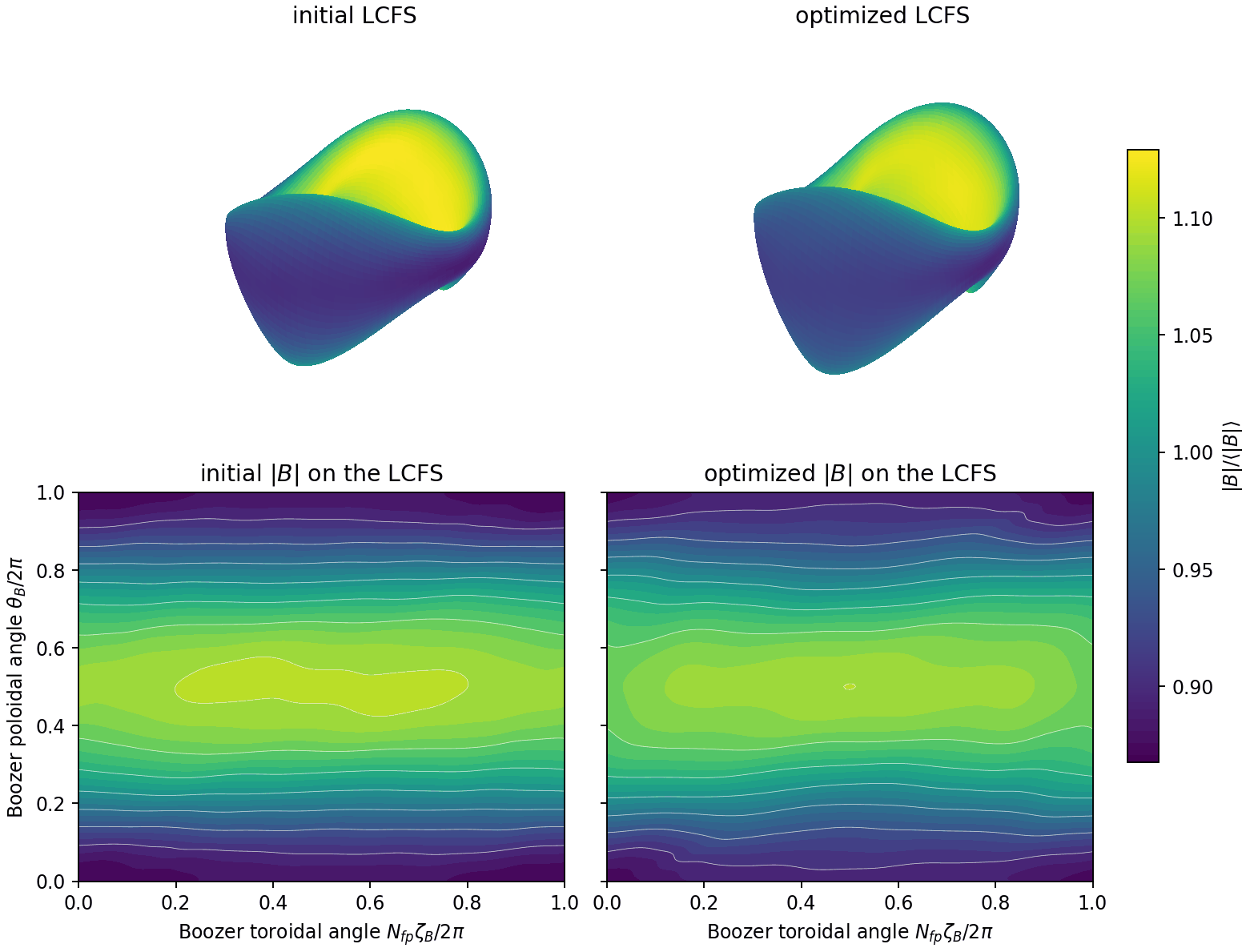
Initial and optimized vacuum equilibria. The 3-D LCFS and Boozer maps use one \(|B|/\langle|B|\rangle\) scale. Eight low-order boundary coefficients move; aspect and mean iota remain within 0.05%.

Forward GKX runs use \(s=0.64\), \(\alpha=0\), (Nx, Ny, Nz, Nl, Nm)=(16,16,24,4,8), Lx=Ly=62.8, and \(\Delta t=0.05\). Each pair shares one fresh random Hermitian multimode state; seeds are independent between pairs. Nominal traces run to \(t=1500\), are sampled every \(\Delta t_s=1\), and average \(1100\leq t\leq1500\).

Uncertainty estimator

For design \(d\in\{b,c\}\), seed \(i\), and \(n\) samples,

\[\bar Q_{d,i}=\frac1n\sum_jQ_{d,i,j},\qquad \rho_{d,i}(k)=\frac{\operatorname{cov}(Q_j,Q_{j+k})} {\operatorname{var}(Q_j)}.\]

GKX integrates \(\rho\) with the trapezoid rule up to its first negative lag [Sokal97]. This positive-window estimator gives

\[\tau_{d,i}=\int_0^{t_{K_0}}\rho_{d,i}(t)\,dt,\qquad n_{eff,d,i}=\min\!\left(n,\frac{n\Delta t_s}{2\tau_{d,i}}\right),\qquad \sigma_{d,i}=\frac{s_{d,i}}{\sqrt{n_{eff,d,i}}}.\]

Matched seeds remove much of the initial-condition variance:

\[r_i=100\left(1-\frac{\bar Q_{c,i}}{\bar Q_{b,i}}\right),\qquad \bar r=\frac1M\sum_i r_i.\]

Two errors are evaluated. The first is the scatter of the \(M\) independent seed-pair reductions. The second propagates the two correlated trace means:

\[\sigma_{pair}=\frac{s_r}{\sqrt M},\qquad \sigma_{IAT}=\frac1M\left[\sum_i100^2\left\{ \left(\frac{\bar Q_{c,i}\sigma_{b,i}}{\bar Q_{b,i}^2}\right)^2 +\left(\frac{\sigma_{c,i}}{\bar Q_{b,i}}\right)^2 \right\}\right]^{1/2}.\]

The reported interval is deliberately conservative,

\[\sigma=\max(\sigma_{pair},\sigma_{IAT}),\qquad \mathrm{CI}_{95}=\bar r\pm t_{0.975,M-1}\sigma.\]

Stationarity is checked on every trace with the half-window shift and linear trend,

\[H=100\frac{\bar Q_2-\bar Q_1}{\bar Q},\qquad S=100\frac{\hat\beta(t_{max}-t_{min})}{\bar Q},\]

where \(\hat\beta\) is the least-squares slope. The final-drift test is \(|S|\leq20\%\), following [Oberparleiter16]. The gate is conjunctive over traces; signed drifts may not cancel across seeds. Heat flux is in gyro-Bohm units.

Matched post-saturation transport

check	pairs	\(\bar Q_b\)	\(\bar Q_c\)	reduction [95% CI]	stationary traces
nominal	24	11.16	9.78	12.26% [10.64, 13.88]	44/48
\(\Delta t=0.04\)	8	11.27	9.58	14.79% [10.52, 19.05]	13/16
\(\Delta t=0.025\)	4	10.76	9.40	12.57% [6.51, 18.64]	7/8
\(N_x=N_y=12\) (coarse)	4	18.73	14.38	23.13% [14.22, 32.04]	7/8
\(N_x=N_y=20\)	16	10.05	9.53	4.95% [2.12, 7.78]	27/32
\(N_x=N_y=24\) (short, rejected)	4	9.27	9.24	0.04% [-14.87, 14.96]	6/8
\(N_x=N_y=24\) (long)	16	9.92	9.07	8.50% [6.34, 10.66]	30/32
\(N_z=16\)	4	10.74	9.76	9.06% [2.37, 15.74]	6/8
\(N_z=32\)	4	11.60	10.15	12.51% [5.76, 19.25]	8/8
\((N_l,N_m)=(3,6)\) (coarse)	4	13.78	11.33	17.12% [0.42, 33.81]	6/8
\((N_l,N_m)=(6,12)\)	16	10.93	9.56	12.32% [9.62, 15.03]	30/32

The intervals above are conditional summaries, not validation intervals. The old gate averaged signed half-window shifts across seeds; opposing drifts cancelled. Applying the published final-drift test independently rejects 4 of 48 nominal traces. Every case except \(N_z=32\) has at least one drift failure, including 2 of 32 long-24x24 and 2 of 32 \((N_l,N_m)=(6,12)\) traces.

The compact raw files contain only \(Q_i(t)\), so neither the increasing high-\(k_y\) tail nor spectral convergence can be tested. Thus none of the 104 matched pairs is promotion-ready. These outputs predate the periodic hypercollision correction and require regeneration: they establish neither transport nor cost for the corrected operator. The 15.32 GPU integration hours on one RTX A4000 describe the historical run only.

Historical initial and candidate ensemble means with seed SEM; the shaded interval is the measured window. Error bars are autocorrelation-corrected conditional summaries. Regeneration with the corrected periodic operator, per-trace stationarity and spectral gates remain open.

VMEX turbulence examples

VMEX ships three QA boundary optimizations that call GKX, in examples/optimization/ of the VMEX repository (pip install 'vmex[turbulence]'). Each adds one GKX objective to VMEX’s QA_optimization.py on flux tubes chosen by s and alpha.

• QA_optimization_turbulence_linear.py: growth rate of the dominant linear ITG eigenmode, with VMEX’s implicit Jacobian through jnp.linalg.eigvals. At s = 0.5 the growth rate went 0.196 to 0.097 (\(v_{ti}/a\)), the aspect ratio 11.5 to 6.4, and the quasisymmetry error rose 0.039 to 0.20. 28 min, 6.5 GB peak.

• QA_optimization_turbulence_quasilinear.py: mixing-length heat flux \(\gamma W_Q/\langle k_\perp^2\rangle\), which needs eigenvector derivatives. The flux went 2.57 to 0.94, aspect ratio 11.5 to 7.7, quasisymmetry error unchanged at 0.04; mean \(|\iota|\) fell to 0.12, below the 0.42 floor these weights do not enforce. 29 min, 6.9 GB peak.

• QA_optimization_turbulence_nonlinear.py: gated saturated heat flux over a finite window, differentiated with the checkpointed discrete adjoint from a fixed saturated start and passed to L-BFGS-B as one scalar. The flux went 53.0 +- 2.6 to 36.3 +- 1.8 after stage 1 and 42.6 +- 2.1 after stage 2, which traded flux for quasisymmetry (error 2.29 to 0.75); aspect ratio 11.5 to 6.0. 70 min, 5.5 GB peak.

Each number is a single run with default settings on a shared 36-core CPU host (12 cores, JAX 0.10.2, GKX 2.4.0, other jobs running). The nonlinear result is one tube and one seed with no held-out check: it shows the pipeline works, not a certified transport reduction.

Reproduce

The workflow has three owners:

• examples/10_vmex_optimization/run.py (formerly QA_optimization.py) computes the VMEX–GKX design step;

• scripts/campaigns/qa_transport_validation.py (retired; Retired generators) runs restartable matched saturation pairs;

• scripts/artifacts/build_qa_transport_figures.py (retired; Retired generators) computes \(\tau_{int}\), effective sample counts, intervals, CSV tables, and plots.

The exact accepted boundaries are initial and optimized. Use a fresh, source-SHA-specific output directory: the campaign skips existing filenames without checking source provenance. Never mix pre-correction and corrected-operator traces. For example,

campaign_dir="campaign/transport-$(git rev-parse --short=12 HEAD)"
python scripts/campaigns/qa_transport_validation.py nominal \
  --seed-stop 24 --output-dir "$campaign_dir"
python scripts/campaigns/qa_transport_validation.py perp24long \
  --seed-stop 16 --output-dir "$campaign_dir"
python scripts/campaigns/qa_transport_validation.py v612 \
  --seed-stop 16 --output-dir "$campaign_dir"
python scripts/artifacts/build_qa_transport_figures.py \
  --raw-dir "$campaign_dir" --output-dir docs/_static

Use the case names and pair counts in the table for the timestep, perpendicular, parallel, and velocity-space scans. Each .npz stores only time, heat_flux, and elapsed seconds. The 208 raw traces stay outside git; their per-trace summary statistics and the plotted nominal mean/SEM are committed. Future promotion runs must also retain content hashes plus \(W_\phi(t)\), \(W_g(t)\), and resolved flux/field spectra.

Download the case summary, per-trace statistics, or nominal time series, or boundary displacement. The Hermite hypercollision exponent follows the resolution-aware min(20, Nm//2) policy.

The derivative mathematics, memory profile, and limitations are in Nonlinear automatic differentiation. Reduced linear and quasilinear objectives remain screening diagnostics, not substitutes for the saturated nonlinear objective.