Examples
The examples directory is a numbered gallery, one directory per workflow;
examples/README.md lists each group with its purpose and runtime. Each
group has a run.py and, where deck-driven, a tutorial case.toml plus the
literature-resolution case_full.toml. Validation decks live in
benchmarks/cases/.
Config-backed runtime cases
These scripts are the closest match to the production benchmark workflows. They load the checked-in runtime TOMLs and expose only the most useful runtime overrides at the command line.
Tokamak cases
python examples/01_linear_tokamak/run.py
python examples/03_nonlinear_tokamak/run.py
gkx benchmarks/cases/etg_linear_scan.toml
gkx benchmarks/cases/kaw_linear.toml
python examples/06_electromagnetic/run.py
gkx benchmarks/cases/kbm_nonlinear.toml
gkx benchmarks/cases/cyclone_nonlinear_miller.toml
VMEC-backed tokamak and stellarator cases
pip install vmec-jax
cd examples/vmec
./generate_wouts.sh
cd ../..

gkx run --config benchmarks/cases/circular_vmec_linear.toml
gkx run --config benchmarks/cases/circular_vmec_nonlinear.toml

gkx run --config examples/02_linear_stellarator/case_full.toml
gkx run --config benchmarks/cases/w7x_linear_quasilinear_vmec.toml
gkx benchmarks/cases/w7x_nonlinear_vmec_geometry.toml
python examples/04_nonlinear_stellarator/run.py
The stellarator tutorial decks run a fixed short window; for production
runs use case_full.toml, which keeps adaptive timesteps enabled.
The bundled VMEC decks are self-contained examples. Exact HSX or W7-X
validation should use the same TOMLs with --vmec-file pointing to the
machine-specific benchmark WOUT. If you only need one local WOUT, run
vmex input.NAME in examples/vmec instead of the full
generate_wouts.sh helper.
The shipped nonlinear stellarator runtime TOMLs write artifact bundles
under tools_out/ by default:
tools_out/w7x_nonlinear_vmec_runtime.diagnostics.csvtools_out/hsx_nonlinear_vmec_runtime.diagnostics.csvtools_out/w7x_nonlinear_imported_runtime.diagnostics.csv
Those diagnostics and their matching *.summary.json files are the intended
inputs for the parity helpers under tools/.
The Python runtime wrappers use the same artifact-aware nonlinear path as the
executable, so long adaptive runs update that bundle as each
chunk completes.
Runtime TOML entry points
When you want the full config surface instead of the thin case wrappers, use the executable or the generic example drivers directly. These runtime utilities are best treated as solver-smoke and exploration entry points; the benchmark examples remain the audited parity surface for ETG and the other validation lanes:
# CASE at the top of the script selects the deck
python examples/12_restart_and_analysis/run.py
python scripts/benchmark.py linear_benchmark etg --outdir tools_out/etg
python scripts/benchmark.py linear_benchmark kbm --outdir tools_out

gkx run-runtime-linear \
  --config examples/08_quasilinear/case_full.toml \
  --out tools_out/cyclone_quasilinear

gkx run-runtime-linear \
  --config benchmarks/cases/w7x_linear_imported_geometry.toml

gkx examples/01_linear_tokamak/case_full.toml
examples/06_electromagnetic/case_full.toml is retained as the canonical operator input for controlled
comparison studies. Its experimental shift-invert path fails closed while the
full-resolution physical residual exceeds the documented acceptance gate; use
the reviewed comparison driver above for the promoted KBM result.
For a bounded runtime-configured independent k_y scan that uses
[parallel] strategy = "batch" without changing the single-k_y solver
layout, run:
python examples/11_parallel_scan/run.py
The companion
examples/11_parallel_scan/case.toml selects two thread
workers through [parallel].num_devices. The runtime still dispatches normal
single-k_y solver calls and gathers results in input order; it does not opt
into the combined-k_y solver path.
Scaling utilities
For production parallelization of independent scans and UQ ensembles, prefer the package helpers:
import jax.numpy as jnp
import gkx as sgk

ky = jnp.asarray([0.1, 0.2, 0.3, 0.4])
chunks = sgk.ky_scan_batches(ky, n_batches=2)
values = sgk.batch_map(
    lambda x: {"gamma": x, "ql_weight": x**2},
    ky,
    batch_size=2,
)
For file-backed calibration and uncertainty workflows that are independent but
not JAX-array vmap workloads, use sgk.independent_map:
rows = sgk.independent_map(
    lambda case: {"case": case, "score": len(case)},
    ["cyclone", "hsx", "w7x"],
    workers=2,
)
These helpers preserve serial ordering and fall back to a one-device vmap
path on laptops. Multi-device runs should still be checked against the serial
result before publication speedups are claimed.
Autodiff validation reports also accept workers for thread-parallel
central finite-difference columns; acceptance is numerical identity with the
serial report.
Parallel identity gates
Each script below writes a JSON sidecar and a figure that compare a parallel
route against the serial or production result it replaces. The ky-scan
figure also reports the observed batch speedup, separately from the identity
check.
Command |
What it compares |
|---|---|
|
Real Cyclone linear solver: serial against fixed-shape |
|
|
|
|
|
|
|
Hermite-sharded |
|
Hermite exchange plus the |
|
Hermite-sharded mirror and curvature/grad-B drift slices (offset-1 and offset-2 Hermite exchanges) against the production linear RHS with only those terms enabled. |
|
Hermite-sharded electrostatic diamagnetic drive: the field-reduction
gate followed by the local |
|
Periodic spectral parallel derivative plus Hermite streaming ladder
through |
|
Streaming-only |
|
Streaming plus electrostatic |
|
Full opt-in electrostatic linear-slices call graph for streaming, mirror, curvature, grad-B, and diamagnetic drive. |
The electrostatic-slices gate is an
opt-in electrostatic linear-RHS identity artifact for the single-species
periodic electrostatic RHS path; collisions, linked boundaries,
electromagnetic terms, and nonlinear brackets are not covered.
For the opt-in Hermite-sharded electrostatic linear RHS path, use the engineering sweep helper:
# retired generator; restore it first: git show f005418bf575:scripts/profiling/profile_linear_rhs_parallel_slices.py > scripts/profiling/profile_linear_rhs_parallel_slices.py
python scripts/profiling/profile_linear_rhs_parallel_slices.py sweep \
  --platform cpu --devices 1,2,4,8 --nms 64,128 \
  --nl 4 --ny 32 --nz 128 --rtol 1e-5
The script writes a device-count and Hermite-resolution sweep figure for the opt-in electrostatic linear-slices backend. The right panel is the identity gate; the left panel is engineering timing only and should not be promoted as a nonlinear or publication speedup claim.
Plotting outputs
To visualize nonlinear diagnostic histories from *.out.nc files:
gkx --plot <output_file>
python examples/12_restart_and_analysis/run.py
Geometry examples
VMEC and Miller geometry usage examples are documented in Geometry.
Nonlinear restart and continuation
The tracked nonlinear runtime path supports a NetCDF out/big/restart
bundle together with continuation from the saved restart state.
One-shot nonlinear bundle write:
gkx run-runtime-nonlinear \
  --config examples/03_nonlinear_tokamak/case_full.toml \
  --steps 200 \
  --out tools_out/cyclone_release.out.nc
For the short Cyclone comparison replay (t_max = 5, no collisions), use
benchmarks/cases/cyclone_nonlinear_short.toml.
That file pins the short-run dissipation contract explicitly
(p_hyper = 2, damp_ends_rate = 0) instead of relying on the longer
production defaults.
Restart-aware TOML snippet:
[time]
nstep_restart = 100

[output]
path = "tools_out/cyclone_release.out.nc"
restart_if_exists = true
save_for_restart = true
append_on_restart = true
restart_with_perturb = false
With that configuration, rerunning the same nonlinear command resumes from
tools_out/cyclone_release.restart.nc when it already exists and appends the
continued history to tools_out/cyclone_release.out.nc. This is the
recommended user-facing workflow for long nonlinear turbulence jobs.
Nonlinear kinetic electrons
examples/05_kinetic_electrons/run.py runs nonlinear turbulence with kinetic
ions and electrons (\(m_e/m_i = 2.7\times10^{-4}\), \(\beta=10^{-4}\))
in the Cyclone base case (case.toml) and in the Landreman-Paul precise QA
stellarator (case_stellarator.toml, a VMEC flux tube at \(s=0.64\)).
python examples/05_kinetic_electrons/run.py
gkx examples/05_kinetic_electrons/case.toml
Choosing dt. Leave fixed_dt = false: the CFL controller takes the
largest linear frequency on the grid. With kinetic electrons that is electron
parallel streaming, \(\sim v_{te}k_{z,\max}\), about
\(\sqrt{m_i/m_e}\approx 60\) times the ion rate. For decks with a light
kinetic species the controller measures the largest eigenvalue of streaming
plus the field solve by a 30-step Arnoldi at startup and takes it when it
exceeds the GX-parity estimate \(v_t k_{z,\max}\max(2\sqrt{N_m},
\omega_H)\). The estimate misses an electromagnetic electron \(m=1\) mode
of the linked box: 702 against 500 on the 16x16x16 tutorial grid at
\(\beta=10^{-4}\) (1604 against 900 at \(10^{-5}\); 454 against 264
on the QA deck), which made the default cfl 0.9 overshoot RK3’s
imaginary-axis interval (\(|\lambda|\Delta t=2.15>\sqrt3\); \(W_g\)
grew \(10^8\) by \(t=0.2\)). The numbers are in
diagnostics.cfl_scales. Measured on the tutorial grid with the default
cfl 0.9:
setting |
controller dt |
outcome |
|---|---|---|
\(\beta=0\) (electrostatic) |
\(3.6\times10^{-4}\) |
stable; the \(\omega_H\) mode at the smallest \(k_\perp\) sets the step |
\(\beta=10^{-5}\) with \(A_\parallel\) |
\(9.6\times10^{-4}\) |
stable to \(t=1\), nonlinear |
\(\beta=10^{-4}\) with \(A_\parallel\) |
\(2.2\times10^{-3}\) |
stable to \(t=1\); six times fewer steps than electrostatic |
\(\beta=10^{-3}\) with \(A_\parallel\) |
\(3.0\times10^{-3}\) |
stable to \(t=1\) |
A small finite \(\beta\) with \(A_\parallel\) is the usual way to remove the electrostatic \(\omega_H\) limit; at \(k_y\rho_i=0.3\) the dominant linear eigenvalue of the tutorial linear deck moves by \(2\times10^{-4}\) between \(\beta=10^{-6}\) and \(10^{-4}\) (0.62478 and 0.62492).
Implicit linear step (opt-in). method = "imex-ars3" with
fixed_dt = true removes the streaming limit. Only the stiff terms are
implicit – parallel streaming with its dissipation (end damping,
hypercollisions, hyperdiffusion), the field response and the electron mirror
force; drifts, the ion mirror and drive stay explicit with the bracket. The
Landau collision operator stays in the RHS, unless it would bound dt
(\(\rho(C)\,\mathrm{d}t > 2\), \(\nu_e \gtrsim 5\) at dt 0.05): then it is
a local backward-Euler sub-step after each step (collision_scheme =
"implicit", the default; "explicit" never uses it). These couple modes only
along one twist-shift chain, and per chain the operator is \(S+UQ\):
\(S\) block-tridiagonal in Hermite with one \(N\times N\) block per
row (\(N\) = links \(\times N_z\); the off-diagonal blocks are the
chain’s parallel-gradient matrix times a ladder scalar) and no species or
Laguerre coupling, and \(Q\) the z-local field solve. GKX probes every
block from the run’s own RHS assembly, factors \(I-\gamma\Delta t S\) by
block Thomas, adds the fields by Woodbury (an equilibrated
\(2N\times2N\) capacitance per chain) and certifies the factor by one
solve’s residual. The step is Ascher-Ruuth-Spiteri ARS(3,4,3): four RHS
evaluations and three solves. Memory is about \((N_m+6)\,n_sN_lN^2\)
complex entries per chain against the dense \((n_sN_lN_mN)^2\): 0.15 GB
at 32x32x16 and 1.5 GB at 64x64x24, both (Nl, Nm) = (4, 8), against 5.5 and
53 GB. Measured on an A4000, against RK3 at its CFL-bound fixed dt, heat
flux averaged over \(t=75\)-150 with 10-unit block errors, both runs
sampled every 0.5:
deck |
step |
\(Q_i\) |
\(Q_e\) |
wall to t = 150 |
|---|---|---|---|---|
Cyclone 64x64x24 (4,8) |
RK3, dt 1.04e-3 |
247 ± 22 |
288 ± 20 |
6883 s |
imex-ars3, dt 0.035 |
270 ± 14 |
310 ± 13 |
678 s (10.1x) |
|
Cyclone 32x32x16 (4,8) |
RK3, dt 1.7e-3 |
538 ± 18 |
674 ± 18 |
491 s |
imex-ars3, dt 0.05 |
533 ± 14 |
672 ± 16 |
113 s (4.4x) |
|
QA 16x16x32 (2,4) |
RK3, dt 3e-3 |
250 ± 17 |
251 ± 16 |
50 s |
imex-ars3, dt 0.05 |
229 ± 16 |
230 ± 15 |
65 s (0.8x) |
The imex walls include building the factor (64 s, 31 s and 30 s). Per step,
an imex step costs 2.7 RK3 steps at 64x64x24 and 2.9 at 32x32x16, so the
stepping alone is 12.5x and 10x faster; on the small decks the build and
compilation dominate, and on the QA tutorial grid RK3 is faster outright.
Linear growth (dominant mode, nonlinear term off, fit over \(t=15\)-20)
agrees with RK3 to \(1.4\times10^{-4}\), \(3.7\times10^{-4}\) and
\(4.1\times10^{-4}\). dt is set by the explicit terms, mostly the
bracket: 0.05 went non-finite at \(t=15\) at 64x64x24 (0.035 and 0.025
are stable) and 0.1 at \(t=1.9\) at 32x32x16. Limits: fixed dt only (one
factor per dt); derivatives flow through the solve with respect to the state
but not through the factors with respect to parameters; production grids
need XLA_PYTHON_CLIENT_PREALLOCATE=false (the factors are captured as
constants of the compiled scan, and with the default 75% preallocation the
64x64x24 executable fails to load). With the electron mirror implicit the
electron blocks couple Laguerre moments (\(N_l N\) square, \(N_l\)
times the memory); the linear step map is then stable to \(\Delta t\approx1\)
(0.05 before), and the nonlinear bracket sets dt instead: 0.1 is stable at
32x32x16 and 0.07 at 64x64x16, (4, 8), where 0.2 and 0.1 went non-finite at
\(t=24\) and 15.6.
Choosing t_max (units of \(a/v_{ti}\)): the linear phase lasts about
\(10/\gamma\), 20-40 here; saturation follows by \(t\approx60\)-100;
then average the flux over at least 100-200 more, or set
run_to = "saturation" to stop once the mean has converged.
Resolution. The tutorial decks use (Nl, Nm) = (2, 4) and 16x16 in the plane. Production runs use 64-96 points in x and y, Nz = 24-64, Nl = 4 and Nm = 8-16 on a GPU; check the heat flux against the next Nm before quoting it.
For linear growth rates use solver = "krylov": the eigen solve has no time
step, so the electron-streaming CFL does not apply.
Lightweight turbulence movies
First persist the production state and its saturation verdict:
python scripts/campaigns/nonlinear_saturated_state.py \
  --toml CASE.toml --state-out saturated_state.npz \
  --output saturation.json
Then run a short production-policy continuation and render it off-device:
python scripts/artifacts/build_turbulence_movie.py CASE.toml \
  --initial-state saturated_state.npz --frames 60 \
  --steps-per-frame 40 --snapshots movie_cuts.npz
python scripts/artifacts/build_turbulence_movie.py \
  --render-from movie_cuts.npz --output turbulence.mp4 --fps 10
Each chunk uses the deck’s explicit method and timestep policy, \(\Delta t_n=P_{\rm CFL}(\phi_n;\Delta t_{\min},\Delta t_{\max},c_{\rm CFL})\). Frame times remain absolute, \(t_k=t_{\rm state}+\sum_{n=1}^{kN_f}\Delta t_n\). The snapshot stores only
so its per-frame payload is \(N_xN_y+N_yN_z\), rather than
\(N_xN_yN_z\). At 96x96x48 this is a 32-fold reduction. Schema 3 also
records the source path and saturation flag, method, fixed/adaptive policy,
resolution, VMEC field-line coordinates, and physical perpendicular extent.
Imported-geometry movies require finite R(z), Z(z), and
zeta(z) profiles and fail instead of drawing an analytic torus when they
are absent. A finite stellarator flux-tube segment is generally open in
three-dimensional space: its endpoints need not coincide. The linked boundary
identifies the gyrokinetic fields through twist-and-shift, not by closing the
centreline in Cartesian coordinates.
Rendering never holds a GPU allocation. A seed-only movie is allowed but is
labelled seeded continuation and is not saturation evidence.
Geometry generation workflows
The runtime geometry path generates imported geometry files from VMEC or
Miller inputs. VMEC uses the booz_xform_jax bridge installed with GKX;
Miller uses the in-package backend:
cd examples/vmec
vmex input.NuhrenbergZille_1988_QHS
cd ../..
gkx geometry vmec \
  --config examples/04_nonlinear_stellarator/case_full.toml

gkx geometry miller \
  --config benchmarks/cases/cyclone_nonlinear_miller.toml
Benchmark and scan helpers
These scripts produce the scan-level plots and tables used in the benchmark discussion:
python scripts/benchmark.py linear_benchmark cyclone
python scripts/benchmark.py linear_benchmark etg
python scripts/benchmark.py linear_benchmark kbm
python scripts/benchmark.py linear_benchmark kinetic
python scripts/benchmark.py linear_benchmark tem
linear_benchmark kbm plots the reviewed fixed-beta ky table. The
matched rerun and branch-continuity analysis live in
scripts/comparison/compare_gx_kbm.py (retired; Retired generators).
The kinetic-electron script loads
examples/05_kinetic_electrons/case_full.toml. The same input
can be run directly with
gkx examples/05_kinetic_electrons/case_full.toml.
It runs on the native RK4 owner.
The TEM script loads benchmarks/cases/tem_linear.toml; users
can run the same single-mode case directly with
gkx benchmarks/cases/tem_linear.toml.
It runs on the native RK2 owner.
Foundational demos
These smaller examples are useful for understanding the numerical building blocks without running a full benchmark case:
# retired generator; restore it first: git show f005418bf575:scripts/benchmarks/basis_orthonormality.py > scripts/benchmarks/basis_orthonormality.py
python scripts/benchmarks/basis_orthonormality.py
python examples/09_autodiff/run.py
python examples/08_quasilinear/implicit_sensitivity.py
Differentiable optimization examples
The public optimization example is a VMEX QA stellarator workflow with one physical GKX heat-flux tuple appended to the objective list:
python examples/10_vmex_optimization/run.py
run.py (formerly QA_optimization.py) mirrors VMEX’s boundary-mode ladder, preserves its
A=6 and mean-iota=0.42 targets, and adds the checkpointed nonlinear
heat-flux derivative. The equilibrium is vacuum; finite a/L_T and a/L_n
drive GKX. Edit the top-level constants to set resolution and run length.
The optimizer window starts from a detached saturated state and supplies a local design derivative. Historical matched runs give a preliminary 12.26% nominal reduction (conditional 95% CI 10.64–13.88%). This is not statistically resolved: individual drift failures and missing resolved spectra block promotion. These traces predate the periodic hypercollision correction and must be regenerated before evaluating current-operator transport. See Stellarator optimization for the audit, resolution ladder, and CSV data.
The reduced synthetic stellarator-ITG diagnostic scripts were retired from
examples/ after GKX 2.3.0 (recoverable from commit f9485f044); their
tracked JSON sidecars under docs/_static remain as historical records.
The production bridge exposes the same portfolio layout for real
vmex -> booz_xform_jax -> GKX rows:
stellarator_itg_vmec_boozer_sample_objective_table_from_state returns a
(surface, alpha, ky, objective) table and
stellarator_itg_vmec_boozer_portfolio_objective_from_state reduces it with
the same weights as the cheap gate. Promotion still requires held-out
surface/field-line artifacts and matched baseline/optimized long
post-transient nonlinear windows, not startup traces or reduced-window
estimators.
examples/09_autodiff/run.py writes a summary JSON and sweep CSVs beside the
figure. One observed mode does not identify both gradients; two modes do,
which is why the gallery uses the two-mode construction.
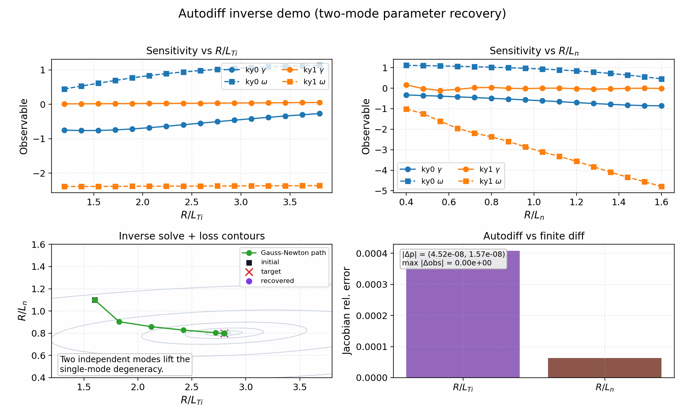
Two-mode inverse validation. The goal is to recover the planted gradients from two independent mode observables and verify that the autodiff Jacobian stays consistent with finite differences. The shipped result reaches the target to numerical precision and is the reviewer-facing parameter-recovery validation.
Secondary slab workflow
gkx run-runtime-linear \
  --config benchmarks/cases/secondary_slab.toml

python scripts/benchmarks/secondary_slab_workflow.py
The staged helper runs the linear seed, writes a restart state in the runtime binary layout, and then launches the nonlinear follow-up with the matching restart and fixed-mode controls used in the tracked secondary benchmark.
Full-GK ETG nonlinear pilot
JAX_ENABLE_X64=1 gkx benchmarks/cases/etg_nonlinear.toml --steps 200
This is the full-GK two-species ETG nonlinear pilot lane. The shipped deck
uses the audited short-window startup contract: Lx = 1.25 for the linked ETG box and
gaussian_init = true with init_single = false because GX reads
init_single from its [Expert] section, not from [Initialization].