Operators And Terms

This page states the operator GKX integrates, term by term, and ties each term to its runtime controls and source files. For TOML syntax and every supported key, see Input Files and Executable.

State And Coupled Variable

For each species \(s\), GKX evolves Laguerre-Hermite moments \(G^{(s)}_{\ell m}(k_x,k_y,z,t)\). The field-coupled variable used by the linear operator is

\[H_{\ell m}^{(s)} = G_{\ell m}^{(s)} + \frac{Z_s}{T_s} J_\ell \phi \,\delta_{m0} - \frac{Z_s v_{th,s}}{T_s} J_\ell A_\parallel \,\delta_{m1} + J_\ell^B B_\parallel \,\delta_{m0},\]

with \(J_\ell^B = J_\ell + J_{\ell-1}\).

On the explicit-time reference-compatible path, streaming acts on the field-coupled streamed variable built from the same field terms before the Hermite ladder is taken.

Source mapping:

src/gkx/operators/linear/params.py (LinearParams)
src/gkx/terms/fields.py
src/gkx/terms/assembly.py

Implemented Linear Operator

The assembled RHS is

\[\partial_t G = \mathcal{R}_{stream} + \mathcal{R}_{mirror} + \mathcal{R}_{curv} + \mathcal{R}_{gradB} + \mathcal{R}_{dia} + \mathcal{R}_{coll} + \mathcal{R}_{hyper} + \mathcal{R}_{k_\perp\text{-hyper}} + \mathcal{R}_{end}.\]

Every term has a multiplicative weight of the same name in TermConfig and RuntimeTermsConfig. All default to 1 except hyperdiffusion and nonlinear, which default to 0.

Gyroaverage And Bessel Factors

The Laguerre gyroaverage coefficients are

\[J_\ell(b) = \frac{1}{\ell!}\left(-\frac{b}{2}\right)^\ell e^{-b/2}, \qquad b = k_\perp^2 \rho_s^2.\]

Nonlinear electromagnetic terms also use \(J_0(\alpha)\) and \(J_1(\alpha)\) on the quadrature grid.

Source mapping:

src/gkx/core_velocity.py
src/gkx/terms/nonlinear.py

Streaming

The Hermite ladder streaming term is

\[\mathcal{R}_{stream} = -w_{stream}\,k_\parallel v_{th,s} \left(\sqrt{m+1}\,X_{\ell,m+1} + \sqrt{m}\,X_{\ell,m-1}\right),\]

where \(X\) is either \(H\) or the benchmark-compatible streamed variable, depending on the solver path.

Controls:

LinearParams.kpar_scale
RuntimeTermsConfig.streaming
boundary/link metadata from the geometry/grid

The parallel FFT uses the signed frequencies of NumPy’s DFT convention. For a chain of \(N\) points separated by \(\Delta z\),

\[D_z e^{2\pi i m j/N} = \frac{2\pi i m}{N\Delta z}e^{2\pi i m j/N}, \qquad k_{N/2}=-\frac{\pi}{\Delta z}\quad(N\text{ even}).\]

Opposite Nyquist signs give the same sampled wave \((-1)^j\) but opposite first derivatives. Match this convention before comparing another code’s RHS; filtering a mode is not a substitute for spatial convergence. Linked chains must use the total chain length and preserve their gather/scatter ordering. test_fft_highest_modes_and_ad_contract checks analytic derivatives, JVPs and real-parameter pullbacks on odd/even periodic and reordered linked chains. The linked-map tests independently check signed frequencies and exact topology. These are discrete-operator contracts, not turbulent-transport benchmarks.

Mirror

The mirror term uses \(b'(z)\) and couples both Laguerre and Hermite indices:

\[\mathcal{R}_{mirror} = -w_{mirror}\,v_{th,s}\,b'(z)\, \Big[ -\sqrt{m+1}(\ell+1)H_{\ell,m+1} -\sqrt{m+1}\ell H_{\ell-1,m+1} +\sqrt{m}\ell H_{\ell,m-1} +\sqrt{m}(\ell+1)H_{\ell+1,m-1} \Big].\]

Curvature And Grad-B

The drift terms are

\[\mathcal{R}_{curv} = - i\,w_{curv}\,\tau_z\,\omega_d\,c_v(z) \Big[ \sqrt{(m+1)(m+2)}H_{\ell,m+2} + (2m+1)H_{\ell m} + \sqrt{m(m-1)}H_{\ell,m-2} \Big],\]

\[\mathcal{R}_{gradB} = - i\,w_{gradB}\,\tau_z\,\omega_d\,g_b(z) \Big[ (\ell+1)H_{\ell+1,m} + (2\ell+1)H_{\ell m} + \ell H_{\ell-1,m} \Big].\]

Controls:

LinearParams.omega_d_scale
RuntimeTermsConfig.curvature
RuntimeTermsConfig.gradb

Diamagnetic Drive

The diamagnetic drive acts through density and temperature-gradient couplings in the low Hermite moments. It drives:

m=0 through density and perpendicular-energy combinations,
m=2 through temperature-gradient coupling,
m=1 and m=3 for electromagnetic A_parallel terms when enabled.

Controls:

LinearParams.omega_star_scale
LinearParams.fprim
LinearParams.tprim
RuntimeTermsConfig.diamagnetic

Collisions

GKX ships six collision models. The collision_operator key in the [time] section of a TOML input selects one, and gkx.operators.linear.collision_tables.collision_operator_from_config() builds the same operator from Python:

`collision_operator`	Model	Reference
`landau` (default)	Linearized Landau (Fokker-Planck), drift-kinetic limit, any `(Nl, Nm)`	built in, described below
`none`, `lenard_bernstein`	Conserving diagonal Lenard-Bernstein/Dougherty relaxation	built in, described below
`sugama`	Drift-kinetic Sugama, conservative by construction	Frei, Ernst & Ricci (2022), Eqs. (C6a)–(C6f)
`improved_sugama`	Improved Sugama, corrected Pfirsch-Schlüter friction	Sugama et al. (2019); Frei, Ernst & Ricci (2022)
`coulomb`	Alias of `landau`. The eight-moment table of Frei, Ernst & Ricci (2022), Eqs. (C9a)–(C9f), it replaced is the same operator with twice GKX’s collision frequency	shipped data kept as a regression reference
`coulomb_finite_kperp`	Gyrokinetic Coulomb retaining finite \(k_\perp\)	Frei, Ball, Hoffmann, Jorge, Ricci & Stenger (2021), Eqs. (3.47)–(3.50)

landau, none and lenard_bernstein are applied inside the linear RHS from the cache, so every solver path (fixed-step, CFL-controlled, Krylov, IMEX, nonlinear) uses them; Hermite-sharded runs refuse landau. none and lenard_bernstein keep the built-in diagonal term described in this section. The three moment operators replace that term with a dense Hermite-Laguerre matrix. The solver switches the diagonal contribution off exactly when a moment operator is active, so collisions are never counted twice.

Two constraints follow from the tabulated coefficients. The run’s basis must be a shipped table’s (Nl, Nm) = (J+1, P+1): (2, 4) for the eight-moment tables, or (3, 6) for the 18-moment finite-Larmor table. Matching Nl*Nm is not enough: the tables are Hermite-major, so the transposed (4, 2) would pair every coefficient with the wrong moment, and it is refused. The operators run on the fixed-step cached integrator. The sharded, Krylov eigenvalue, and CFL-controlled explicit_time paths raise rather than silently substituting the diagonal term. The Coulomb tables are generated at unit mass and temperature ratio, so a multispecies request is refused rather than extrapolated.

Linearized Landau operator (default)

The default is the linearized Landau operator about Maxwellians, \(C_{ab}[f_a,f_b]=C(f_a,F_b)+C(F_a,f_b)\), in its drift-kinetic (\(k_\perp\to0\)) limit, applied to the non-adiabatic response H. With \(x=v/v_{ta}\), \(v_{ta}=\sqrt{2T_a/m_a}\), the test part is the Rosenbluth diffusion

\[C(f_a,F_b) = \nu_{ab}\,\nabla\cdot\Big[\tfrac12 \mathsf D_b\cdot\nabla f_a - \tfrac{m_a}{m_b}\,f_a\nabla H_b\Big],\qquad \nu_D^{ab}(x)=\nu_{ab}\,\frac{\operatorname{erf}(x_b)-G(x_b)}{x^3},\]

with \(G\) the Chandrasekhar function and \(H_b\), \(\mathsf D_b=\nabla\nabla G_b\) the Rosenbluth potentials of \(F_b\). The field part is

\[C(F_a,f_b)=\nu_{ab}F_a\Big[4\pi\tfrac{m_a}{m_b}f_b-\alpha H_b +\big(\tfrac{m_a}{m_b}-1\big)\alpha\,v\,\partial_v H_b +\tfrac12\alpha^2 v_iv_j\partial_i\partial_j G_b\Big],\qquad \alpha=m_a/T_a,\]

with \(H_b\), \(G_b\) the potentials of the perturbation \(f_b\) (Helander & Sigmar 2002, ch. 3). The operator is rotationally invariant, so in the Legendre-Sonine basis \(x^lL_k^{(l+1/2)}(x^2)P_l(\xi)\) it is block diagonal in \(l\) and each block is a pair of radial integrals. GKX evaluates them by composite Gauss quadrature once per run, for the run’s (Nl, Nm) and species mass and temperature ratios, and maps them to the Hermite-Laguerre box with an exact orthogonal transform (gkx.operators.linear.collisions.linearized_landau_pair_matrices()). The result is a dense matrix per species pair; one RHS applies it as a moment-space matrix product.

What is verified (tests/validation/physics_gates/test_collision_physics.py):

density, parallel momentum and energy are exact null vectors (1e-13), the like-species matrix is symmetric negative semidefinite with exactly three zero eigenvalues (H-theorem);
it equals the multiprecision Coulomb tables of Frei et al. (2021, 2022) to 1e-12 at (Nl, Nm) = (2, 4) and (3, 6), once their collision frequency (twice GKX’s) is accounted for;
its test part equals the Sugama test part at equal temperatures for \(m_a/m_b = 1,\ 1/1836,\ 1836\);
electron-ion momentum and energy exchange cancel exactly, also at \(T_e/T_i=3\);
the Spitzer-Harm ratio \(\gamma_E(Z)\) is within 0.5% of Spitzer & Harm (1953) for \(Z=1,2,4,16\);
the application is differentiable in nu (and in density and charge).

Frequency convention. nu is each species’ self-collision frequency in GKX units, \(\nu=\sqrt2\,\mathtt{vnewk}^{\rm GS2}\), and \(\nu_{ab}=\nu_a n_bZ_b^2/(n_aZ_a^2)\). Inter-species conservation is exact when the species rates are mutually consistent, \(\nu_a\propto n_aZ_a^4/(m_a^{1/2}T_a^{3/2})\). At unequal temperatures the operator still conserves but is not self-adjoint; the thermal equilibration \(C(F_a,F_b)\) is dropped, as in all delta-f codes.

Default and cost. landau is the default both in the runtime and in LinearParams (collision_model); the matrices are built only when some nu is nonzero. The runtime applies the factors \(T B T^{\mathsf T}\) directly: \(T\) is block diagonal in the degree \(p+2j\) and \(B\) in \(l\), which at \((N_l,N_m)=(16,48)\) is 4.1x fewer flops than the dense product. On an idle A4000, Cyclone grid \(16\times8\times32\), the whole linear RHS at \((16,48)\) costs 1.6x the Dougherty RHS in float32 (one and two species) and 1.9x (one species) and 2.3x (two species) in float64; at \((8,24)\), 1.4-1.7x (plan/research/2026-10-15-collisions/results/rhs_collision_share_gpu.txt).

Benchmarks against other codes (results/xcode_collisional.txt, results/zonal_collisional.txt):

Cyclone ITG with adiabatic electrons, \(k_y=0.3\), \(\nu_i\) from 0 to 0.1: within 1.1% of GS2’s model operator at \((N_l,N_m)=(12,48)\), including GS2’s slight collisional destabilisation. The Dougherty kernel goes the other way, and is 21% low at \(\nu_i=0.1\).
Cyclone with kinetic electrons (\(m_e/m_i=2.7\times10^{-4}\)), \(\nu_i\) from 0 to 0.1 with consistent \(\nu_e\): within 1.2-4.8% of GS2 at \((8,24)\). Dougherty is 11% low at \(\nu_i=0.03\).
Collisional decay of the Rosenbluth-Hinton residual (s-alpha, \(q=1.4\), \(\epsilon=0.18\)): the residual levels are within 6% of Xiao, Catto & Molvig (2007), but the decay rate is 21-27% slower. That formula drops energy diffusion, and its \(\nu_{ii}\) convention was not checked against the paper, so the rate is not used as a gate. The Dougherty kernel does not damp this residual at all.

Not included: finite-\(k_\perp\) (gyroaveraging) terms, which coulomb_finite_kperp carries for one species at fixed tabulated resolutions. The matrix depends on mass and temperature ratios through a host-side build, so it is not differentiated with respect to them.

Collision frequency

The tabulated matrices carry only the dimensionless pair scaling \(\nu_{ab} = n_b / (\sqrt{m_a}\,T_a^{3/2})\). The common collisionality prefactor comes from the species nu, so every model sits on the same collisionality axis as the built-in Lenard-Bernstein term.

Warning

Three mutually incompatible normalizations of the collision frequency appear in this literature. Writing \(\nu = C\,n q^4 \ln\Lambda / (m^{1/2} T^{3/2})\), Sugama (2009, 2019) uses \(C = 4.4429\), Frei et al. (2021) and Frei, Ernst & Ricci (2022) use \(C = 2.3633\), and Frei, Hoffmann & Ricci (2022) use \(C = 0.7523\). Any comparison against a published figure must fix the convention first; it is the most common source of apparent agreement.

Baseline Lenard-Bernstein model

The built-in collisional model is a Lenard-Bernstein-style diagonal damping plus conservation-restoring low-order moment corrections. The base damping is

\[\mathcal{R}_{coll}^{base} = - w_{coll}\,\nu_s\,\Lambda_{\ell m}\,H_{\ell m},\]

where lb_lam is the cached Hermite/Laguerre collision eigenvalue, \(\Lambda_{\ell m} = \nu_\ell\,\ell + \nu_m\,m\) with nu_laguerre (default 2) and nu_hermite (default 1). The code then reconstructs the low moments

\[\bar{u}_\perp = \sqrt{b}\sum_\ell J_\ell^B H_{\ell,0}, \qquad \bar{u}_\parallel = \sum_\ell J_\ell H_{\ell,1},\]

and a temperature-like correction \(\bar{T}\) from m=0 and m=2, and adds them back only into the m=0,1,2 channels.

This is a conserving Lenard–Bernstein/Dougherty-like model, not a complete linearized gyrokinetic Landau operator. Its low-order field-particle correction matters: the operator cannot be represented by a diagonal damping array alone.

At \(k_\perp\rho=0\) the model conserves each species’ density, parallel momentum and temperature-like moments; a five-step gate checks this from populated high moments, in serial and decomposed integration. At finite \(k_\perp\rho\) the guiding-centre moments are not locally conserved. Collisions are local in real space, so the gyrocentre change is nonlocal. This is the physics of the published model, not a residual to tune away. A direct finite-\(b\) gate checks every term of equations (3.38)–(3.42) of Frei et al. (2021), including parallel/perpendicular flow and temperature restoration.

Structural verification of the moment operators

Every shipped matrix is asserted against the published closed forms, not only against internal consistency. All twelve Appendix-C coefficients of Frei, Ernst & Ricci (2022) (six Coulomb, six Sugama) reproduce, for example

\[C^{(1,1)}_{(1,1)} = -\frac{28}{15}\sqrt{\frac{2}{\pi}}, \qquad C^{(3,0)}_{(1,1)} = -\frac{8}{5}\sqrt{\frac{1}{3\pi}} .\]

GKX stores the opposite Laguerre sign convention to the paper, so a published entry maps onto the stored one through \((-1)^{j+j'}\). That flips exactly the couplings between different Laguerre parities and leaves same-parity entries alone, so the comparison checks the convention as well as the values.

tests/validation/physics_gates/test_collision_physics.py gates the properties a linearized collision operator must satisfy. The offline verification artifact docs/_static/collision_operator_verification.json records the measured values against its thresholds:

Property	Measured	Gate
Density, parallel-momentum, energy conservation	\(5.6\times10^{-17}\)	\(5\times10^{-12}\)
H-theorem (largest eigenvalue of the symmetrized operator)	\(9.0\times10^{-18}\)	\(10^{-12}\)
Onsager self-adjointness	\(8.3\times10^{-17}\)	\(5\times10^{-12}\)
Published Appendix-C coefficients	\(1.1\times10^{-16}\)	\(5\times10^{-12}\)
Finite-Larmor gyrocenter-diffusion order at small \(b\)	\(B^{1.94}\)–\(B^{2.00}\)	\(B^{1.7}\)–\(B^{2.3}\)

The invariants are the left null vectors of the moment matrix, since the production of a moment functional \(v\) is \(v^{T} C N\). With the Hermite-major index \(p(J+1)+j\) they are \(e_0\) (density), \(e_2\) (parallel momentum), and \(e_1 + e_4/\sqrt{2}\) (energy), the last read off the exact null space rather than assumed. At \(b=0\) the finite-Larmor tables reduce to the drift-kinetic Coulomb operator.

The finite-Larmor operator acts on gyrocenter moments. Gyroaveraging modifies their conservation and plain self-adjointness, so the test is the ordering: both defects must vanish at \(b=0\) and enter at first order in \(b = B^2/2\). A kernel assembled at the wrong order would show \(B^{1}\) or \(B^{4}\) instead. The finite-\(b\) density row is classical gyro-diffusion, not a conservation failure. Equation (3.35) of Frei et al. (2021) maps a gyrocenter distribution to particle moments; it does not invert the gyrophase average of equation (3.5), so local particle-space conservation cannot be inferred by applying that map to the gyroaveraged collision matrix.

Tabulated resolutions

Finite-Larmor tables ship at 8 and 18 Hermite-Laguerre moments. They are generated in 60-digit arithmetic on a 14-point Bessel-argument grid \(B = k_\perp v_{\mathrm{th}}/\Omega \in [0, 4]\) and stored as checksummed float64. The runtime interpolates at \(B=\sqrt{2b}\) from the cached \(b\), so one table covers every perpendicular wavenumber, and it selects the table matching the run’s Nl*Nm automatically, then requires the run’s (Nl, Nm) to be that table’s (J+1, P+1).

Cost and the resolution ceiling

The finite-Larmor operator interpolates its tables at every grid point, so the compiler sees a distinct moment matrix per \((k_y, k_x, z)\). That storage grows as \(n^2\) in the moment count \(n\) while the state grows as \(n\). On a 16x8x32 grid the compiled linear RHS needs 5.9x the temporary storage of the built-in diagonal operator at 8 moments and 12.1x at 18. The cost gates in test_collision_physics.py bound these ratios at 12x and 24x, and bound the growth between the two resolutions by the \(n^2\) ratio.

Extrapolating the per-point matrices to a 32x64x32 grid gives:

moments `Nl*Nm`	per-point matrix storage	note
8	0.07 GB	shipped
18	0.34 GB	shipped
128	17 GB	linear Cyclone ITG convergence resolution; exceeds a 16 GB card
512	275 GB	converged resolution in the published study

The published convergence resolutions are therefore not reachable in this form, and resolution should be scanned rather than assumed. Generate a further table resolution with:

python scripts/artifacts/build_finite_wavelength_coulomb_data.py \
    --hermite 7 --laguerre 3 --digits 60 --workers 24 --check

Python collision protocol

A collision model receives a post-field CollisionContext (distribution, hamiltonian, fields, cache, parameters; see src/gkx/operators/collision.py), so finite-Larmor models can distinguish the evolved distribution \(G\) from the Hamiltonian response \(H\). It implements

apply(context), the complete unit-weight RHS, including low-rank or dense field-particle terms; and optionally
SplitCollisionOperator.split_step(context, dt), an exact or implicit finite-time update. The runtime does not route this method.

Pass the model to linear_rhs_cached or nonlinear_rhs_cached with collision_operator=. The callback must return a JAX array with the state shape. GKX removes the built-in collision contribution before adding terms.collisions * operator.apply(...); hypercollisions stay independent:

class CollisionModel:
    def apply(self, context):
        return collision_rhs(
            context.distribution,
            context.hamiltonian,
            context.cache,
            context.parameters,
        )

rhs, fields = nonlinear_rhs_cached(
    state, cache, parameters, terms,
    collision_operator=CollisionModel(),
)

The callback runs after the field solve and is traced by JAX, so its array operations stay differentiable. context.fields carries phi, apar, and bpar; context.hamiltonian follows the same enabled-field policy as the gyrokinetic RHS.

The [time] collision_split policy splits only diagonal hypercollisions. The conserving collision term stays in the Runge–Kutta RHS, with its field-particle corrections; the chain IMEX steps (imex-ars3, imex-ark3) advance the Landau operator by a local backward-Euler sub-step instead (collision_scheme = "implicit") when the explicit collision bound would bind, which removes \(\nu_e\) from the step-size bound (Resolution, Step and Solver Guidance).

Diagnostics in src/gkx/operators/linear/dissipation.py:

collision_invariant_rates returns the discrete long-wavelength density, parallel-momentum, and thermal-energy rates of a state-shaped contribution.
collision_quadratic_rate evaluates \(\operatorname{Re}\langle H,C[H]\rangle\) with optional species/spatial weights.
multispecies_collision_invariant_rates returns each species’ particle rate and the weighted sums

\[\dot P_\parallel = \sum_s n_s\sqrt{m_s T_s}\,\dot N_s^{10}, \qquad \dot E = \sum_s n_s T_s \left(\sqrt{2}\,\dot N_s^{20}+2\dot N_s^{01}\right),\]

which must all vanish for a species-coupled model.

Research operators (Python only)

The following are exported from gkx.operators.linear (or the module named) for verification and model development. None of them has a TOML selector.

API	What it is
`drift_kinetic_sugama_six_moment_contribution`	The like-species six-gyromoment Sugama matrix of Appendix C, Eqs. (C6a)–(C6f); zero outside the six-moment projection.
`load_collision_moment_matrix`, `apply_collision_moment_matrix`, `interpolate_collision_moment_matrix`, `apply_multispecies_collision_moment_matrix`	Checksummed package-data tables and their JAX application, including per-species and ordered target/source pair tables interpolated in \(k_\perp\) on device.
`drift_kinetic_sugama_pair_matrices`, `drift_kinetic_improved_sugama_pair_matrices`, `assemble_drift_kinetic_sugama_matrix`, `assemble_drift_kinetic_improved_sugama_matrix`, `DriftKineticMomentCollisionOperator`	Multispecies drift-kinetic original and improved Sugama on the eight-mode space (Appendix C, Eqs. (C4)–(C5) and (101)–(102)), with directed frequency \(\nu_{ab}\propto n_b/(\sqrt{m_a}T_a^{3/2})\). This is what the `sugama` and `improved_sugama` selectors build.
`TabulatedMultispeciesCollisionOperator`, `FiniteWavelengthCoulombOperator`, `EqualSpeciesFiniteWavelengthCoulombOperator`, `EqualSpeciesFiniteWavelengthSugamaOperator`	Finite-wavelength operators that interpolate generated test, field and polarization tables at \(B_a=\sqrt{2b_a}\). The equal-species forms refuse multispecies input.
`parallel_electric_field_source`, `solve_driven_collision_response`	The driven parallel-current problem \(C N_e + s_E = 0\) of Frei, Ernst & Ricci (2022), Eq. (81), solved with `jax.numpy.linalg.solve`.
`bessel_laguerre_kernels`, `associated_bessel_laguerre_coefficients` (`gkx.core_velocity`)	\(K_n(B) = e^{-B^2/4}(B^2/4)^n/n!\) and the equation-(2.12) prefactor of Frei et al. (2021).
`conservative_full_f_dougherty_cross_moments` (`gkx.operators.nonlinear.collisions`)	The pairwise primitive moments of the improved multispecies Dougherty model (Francisquez et al., Eqs. (2.11)–(2.12)). This is a full-\(f\) reference; it must not be inserted into the linearized field-particle restoration.

The high-precision coefficient algebra (Coulomb speed integrals, basis transforms, Laguerre products and the equation (3.48)–(3.50) contractions) lives in the offline generator scripts/artifacts/build_linear_validation_artifacts.py (retired; Retired generators), not in the package. The runtime only interpolates validated tables and applies matrices, which is the same split as the GYACOMO/COSOlver pair.

References: Frei et al. (2021), Frei, Ernst & Ricci (2022), Abel et al. (2008) (the conservation, null-space, adjointness and H-theorem requirements), Jorge, Ricci & Loureiro (2017) and Jorge, Frei & Ricci (2019) (the basis transforms), and the improved multispecies Dougherty derivation.

Collision validation evidence

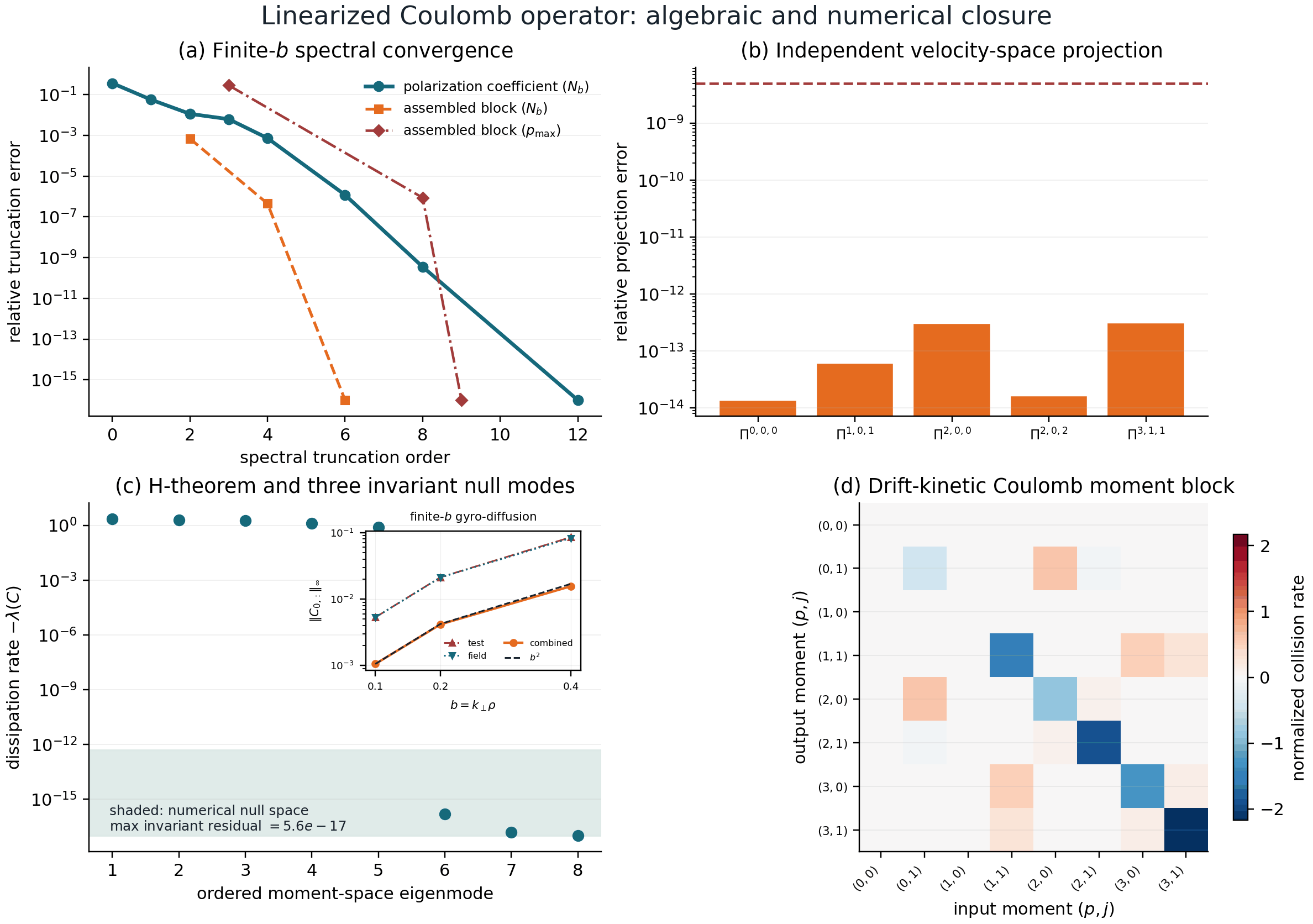
Coulomb collision operator convergence, projection, entropy, and matrix gates — **Offline Coulomb-operator closure.** Panel (a) shows Bessel–Laguerre convergence of a finite-\(b\) polarization coefficient to a 24-term reference, Bessel convergence of an assembled 4-by-4 collision block, and the independent spherical/radial hierarchy convergence of that block; panel (b) compares five generated coefficients with independent 80-by-80 Gauss–Hermite/Laguerre velocity projection; panel (c) shows five dissipative modes and the three density, parallel-momentum, and thermal- energy null modes, while its inset verifies leading \(O(b^2)\) classical gyro-diffusion away from the drift-kinetic limit; panel (d) shows the complete retained drift-kinetic moment block. The machine-readable gate is `collision_operator_verification.json`.

Regenerate with python scripts/artifacts/build_linear_validation_artifacts.py collision-verification (retired; Retired generators). The largest direct-projection relative error is \(3.1\times10^{-13}\). At \(b=0.8\) the assembled block changes by \(4.50\times10^{-7}\) between Bessel orders four and six, at the \((p_{\max},j_{\max})=(8,4)\) spherical cutoff, which is within \(8.68\times10^{-7}\) of the \((9,4)\) reference. The smaller cutoff \((3,1)\) differs from that reference by 29% and is rejected.

Driven parallel current. The collision-response subcommand (retired; Retired generators) built docs/_static/collision_response_convergence.json from equations (3.53)–(3.56). With \(\widehat E=eE/(m_ev_{Te}\nu_{ee})\), the plotted response \((u_e/v_{Te})/\widehat E\) is \(\sigma_\parallel/[n_e e^2/(m_e\nu_{ee})]\). At \((P,J)=(20,5)\) the largest current change from \((15,5)\) is \(1.66\times10^{-4}\) over \(Z=1,2,5,10,100\), and the invariant, self-adjointness, spectrum and driven-solve residuals pass a \(2\times10^{-12}\) gate. Original Sugama gives 11.29% less current than Coulomb at \(Z=1\) and 0.61% less at \(Z=100\); improved Sugama stays within 0.307% of Coulomb at every scanned charge. The \(Z=100\) Coulomb point is 7.453% from the Spitzer high-charge limit \(64/[3\,2^{3/2}\pi Z]\), inside the 8% gate. This validates the unmagnetized equal-temperature conductivity problem, not finite-\(b\) collisional transport.

Collisional zonal response. docs/_static/collision_finite_wavelength_zonal_response.json reproduces the Figure 12–14 protocol of Frei, Ernst & Ricci (2022) at P24/J10 through \(t\nu=30\). The late responses are:

\(k_x\rho_i\)	original Sugama	improved Sugama	Coulomb
0.1	0.00242	0.00255	0.00288
0.2	\(9.66\times10^{-5}\)	\(1.15\times10^{-4}\)	\(1.92\times10^{-4}\)

Improved Sugama tracks Coulomb more closely than the original model in the early window at both wavenumbers.

Short-wavelength ITG boundary. On a Cyclone-like s-\(\alpha\) probe, raising the drift-kinetic collision weight damps the growth rate at \(k_y\rho\simeq0.63\) but excites the short-wave branch at \(k_y\rho\simeq0.94\), the behaviour expected when collisional FLR terms are omitted. test_drift_kinetic_collision_model_is_blocked_for_short_wave_itg requires both observations. Only a converged finite-\(b\) operator can close that lane.

Controls:

[time] collision_operator
RuntimePhysicsConfig.collisions
RuntimeTermsConfig.collisions
RuntimeSpeciesConfig.nu
RuntimeCollisionConfig.nu_hermite
RuntimeCollisionConfig.nu_laguerre

For two kinetic species, the explicit species-parallel integrator evaluates the complete built-in collision contribution locally on each device after the shared field reduction; nonzero, unequal ion/electron rates are identity-gated against serial evolution. The direct species-sharded RHS helper is collision-free, so use integrate_linear(..., parallel=RuntimeParallelConfig(strategy="velocity", axis="species", num_devices=2)) for the collisional route. The same route is gated for Hermite/Laguerre hypercollisions with nonzero nu_hyper_l/nu_hyper_m. Electromagnetic species decomposition sums the local field moments over the species axis and reduces them across devices, so phi, apar and bpar are the serial fields; mixed species–Hermite meshes are not covered.

Hypercollisions

GKX implements an isotropic branch, a constant-coefficient Hermite/Laguerre branch, and a \(|k_z|\)-scaled Hermite branch:

\[\mathcal{R}_{hyper}^{const} = -w_{hyper} \Big[ v_{th,s}\big(\tilde{\nu}_\ell r_\ell + \tilde{\nu}_m r_m\big) + \nu_{\ell m} r_{\ell m} \Big]G,\]

\[\mathcal{R}_{hyper}^{iso} = -w_{hyper}\,\nu_{hyper}\,r_{hyper}\,G,\]

\[\mathcal{R}_{hyper}^{|k_z|} \propto -w_{hyper}\,\nu_{k_z}\,|k_z|\,m^{p_m}\,G.\]

Controls, and the branch each one reaches:

`RuntimeCollisionConfig` knob	Branch	Notes
`nu_hyper` / `p_hyper`	isotropic	always applied; defaults `0.0` / `4.0`
`nu_hyper_l` / `p_hyper_l`	constant only	the Laguerre channel. The \(\|k_z\|\) kernel has no \(\ell\) index, so this knob needs `hypercollisions_const = 1`
`nu_hyper_lm` / `p_hyper_lm`	constant only	mixed channel, same restriction
`nu_hyper_m` / `p_hyper_m`	both	the Hermite channel; the constant branch reuses it unless `nu_hyper_m_const` is set
`nu_hyper_m_const`	constant only	per-branch Hermite rate. `None` (default) reuses `nu_hyper_m`; `0.0` gives a pure Laguerre sink beside an unchanged \(\|k_z\|\) Hermite branch, so Hermite is not damped twice
`hypercollisions_const` / `hypercollisions_kz`	branch switches	see the defaults below

The defaults differ between a TOML run and a hand-built LinearParams:

Setting	TOML runtime (`RuntimeCollisionConfig`)	Python `LinearParams`
`hypercollisions_const` / `hypercollisions_kz`	`0.0` / `1.0` (the \(\|k_z\|\) branch, as in the reference code)	`1.0` / `0.0` (the constant branch)
`nu_hyper_m`	`1.0`	`1.0`
`p_hyper_m`	`None`, resolved to \(\min(20, \max(\lfloor N_m/2\rfloor, 1))\)	`20.0`

RuntimePhysicsConfig.hypercollisions and RuntimeTermsConfig.hypercollisions gate the whole operator.

Declared velocity-space regularization

Because nu_hyper_l is branch-bound, a deck that set it under the runtime defaults would have run with no Laguerre sink. That is an error: RuntimeCollisionConfig refuses a nonzero nu_hyper_l or nu_hyper_lm while hypercollisions_const = 0.0, and names the two ways to fix it. Cross-section case validation also refuses those channels when RuntimePhysicsConfig.hypercollisions or RuntimeTermsConfig.hypercollisions disables the whole operator. A declared regularization either acts or the run stops; it is never silently discarded.

This matters beyond configuration hygiene. For the Cyclone s-\(\alpha\) adiabatic-electron ITG mode at \(k_y \rho_i = 0.55\), certified eigenpairs show that the collisionless growth rate is not converged in Laguerre resolution: the eigenvector carries a cutoff pile-up that relocates to 0.79–0.85 of every new Nl instead of resolving, and the only ladder that converges is the one with enough velocity-space dissipation to remove it. A collisionless growth rate at such a point is a truncation value, not a converged number.

Contract. Every collisionless linear row published from GKX declares the velocity-space regularization it used, and reports the \(\nu \to 0\) (or \(\nu_{hyper} \to 0\)) extrapolation rather than a single regularized number. none is a legal declaration and the common one for reference-code parity rows, whose decks must reproduce the reference exactly; it commits the row to being reported as resolution-limited, not as a converged growth rate. The declaration is a required field of every linear row of tools/evidence_ledger.toml and is checked by tests/release/test_release_gates.py.

Hyperdiffusion And End Damping

The perpendicular hyperdiffusion term is

\[\mathcal{R}_{k_\perp\text{-hyper}} = -w_{hyperdiff}\,D_{hyper} \left(\frac{k_\perp^2}{k_{\perp,\max}^2}\right)^{p_{hyper,k_\perp}} G,\]

masked by the dealias region. \(k_{\perp,\max}^2\) is the dealiased corner of the full grid: when a linear run selects a subset of ky rows, the parent grid’s \(|k_y|\) at row (Ny - 1) // 3 is carried as SpectralGrid.ky_cut and used in place of the missing row. D_hyper defaults to 0 and the hyperdiffusion term weight to 0, so it is off unless a deck enables it.

The field-line end damping is \(\mathcal{R}_{end} = -w_{end}\,\nu_{end}\,d(z)\,H\), where \(d(z)\) is a smooth profile over the last damp_ends_widthfrac (default 0.125) of the chain at each end, and zero on a periodic boundary. The zonal row carries no end damping. \(\nu_{end}\) is one timestep-free rate on every route; its default and how to check sensitivity are in Parallel boundary and end damping.

Controls:

RuntimeTermsConfig.hyperdiffusion
RuntimeCollisionConfig.D_hyper
RuntimeCollisionConfig.p_hyper_kperp
[time] damp_ends_rate
RuntimeCollisionConfig.damp_ends_widthfrac

Nonlinear \(E \\times B\) And Flutter

The nonlinear bracket is evaluated pseudospectrally:

\[\{f,g\} = \partial_x f\,\partial_y g - \partial_y f\,\partial_x g.\]

The electrostatic nonlinear term is

\[\mathcal{R}_{NL,E\times B} = -w_{nl}\,\{g,\langle \chi \rangle\},\]

and the electromagnetic flutter contribution couples adjacent Hermite moments:

\[\mathcal{R}_{NL,flutter} = -v_{th,s} \left( \sqrt{m}\,\{\langle A_\parallel \rangle,g\}_{m-1} + \sqrt{m+1}\,\{\langle A_\parallel \rangle,g\}_{m+1} \right).\]

Controls:

TimeConfig.compressed_real_fft (default true)
TimeConfig.laguerre_nonlinear_mode (default "grid")
TimeConfig.nonlinear_dealias (default true, the 2/3 rule)
RuntimeTermsConfig.nonlinear

Source Mapping

linear term kernels: src/gkx/terms/linear_terms.py and src/gkx/operators/linear/
collision models: src/gkx/operators/linear/collisions.py, src/gkx/operators/linear/collision_tables.py, src/gkx/operators/linear/collision_tables.py
nonlinear term kernels: src/gkx/terms/nonlinear.py and src/gkx/operators/nonlinear/
assembly: src/gkx/terms/assembly.py
low-level parameter container: src/gkx/operators/linear/params.py
runtime parameter surface: src/gkx/config.py

Parameter Surface

The primary parameter groups are:

RuntimePhysicsConfig
RuntimeCollisionConfig
RuntimeNormalizationConfig
RuntimeTermsConfig
LinearParams

For TOML syntax and all supported keys, see Input Files and Executable.