Performance

This page covers where a GKX run spends its time on one device, how to profile it, and the tracked profiler artifacts that back each number. Multi-device and multi-worker evidence – independent scans, ensembles, sharded nonlinear routes and their identity gates – is in Parallelization policy.

JAX performance model

GKX uses JAX to compile array kernels ahead of time, enabling vectorized, accelerator-ready performance while retaining automatic differentiation. The linear operator and time integrator are designed to be jit-friendly and to avoid Python-side loops in performance-critical paths.

The linear solver precomputes geometry-dependent arrays (gyroaverage coefficients, drift components, mirror term, and zero-mode masks) in a LinearCache so they are not recomputed at each time step. The cache also stores the Laguerre/Hermite index arrays and their derived coefficients (l+1, m+1, sqrt(m), sqrt(m+1)), which the mirror, curvature and implicit-preconditioner terms reuse instead of rebuilding them on every RHS call. The cache is reused inside the compiled integrator.

The linear integrator is jit-compiled with the number of steps and method as static arguments. The operator term switches (gkx.operators.linear.params.LinearTerms) should remain static inside a compiled loop to avoid recompilation, and the cached operator arrays can be built once and reused across runs. Nonlinear IMEX paths reuse the electrostatic compiled linear-RHS route whenever apar = bpar = 0.

benchmarks/references/gkx_2_representative_performance_refresh.json is the compact representative refresh. It admits two bounded local-CPU rows after finite CPU/GPU numerical checks; its office-GPU timings are kept as rejected provenance because both A4000s were already fully loaded, so they do not update the published speed claim.

Explicit-step kernels

The mirror, curvature and grad-B terms shift H by up to two Hermite and one Laguerre index. XLA lowers every shifted view as its own sweep of the state; at 64x64x24, (Nl, Nm) = (4, 8) in float32 the Laguerre stride is 6 MB against a 4 MB L2 on an RTX A4000, so each view costs a DRAM pass. Those fused RHS kernels ran at 14–60 GB/s of a 448 GB/s peak and were 55 per cent of the explicit step. gkx.terms.linear_terms.fused_drift reads each (l, m) neighbourhood once per tile in a Pallas (Triton) kernel on real and imaginary planes, the form Triton accepts: 0.15 ms for the three terms against 2.2 ms, at round-off agreement with the jnp terms (1.8e-7 relative in float32, 1.7e-16 in float64). It runs on NVIDIA GPUs when Nx*Nz >= 64 and Nl*Nm <= 256; CPU, other GPUs, Hermite-sharded slabs and the per-term diagnostics keep the jnp terms, which are also what forward- and reverse-mode derivatives go through.

Two smaller changes apply on every backend. The jnp terms slice one padded copy of H instead of padding per shift, which on XLA:CPU removes the recomputation of H in each view (bitwise identical). The Nyquist fix of the linked streaming output touches the two self-conjugate rows rather than reducing over the whole state (bitwise identical; the stacked streaming and hypercollision transform at (8, 16) went from 5.6 to 3.6 ms on GPU). It is a concatenate on GPU and an in-place scatter on CPU, where XLA turns the concatenate into a copy fusion twice as slow as the whole-state version. On XLA:CPU the linked output is also materialized before the conjugate restore, which otherwise fuses the gather into the restore and recomputes it; on GPU that barrier costs 30 per cent and is not applied.

Running on CPU

A shipped default deck at 96x96x48 takes roughly 1.1–1.6 hours on an Apple M3 Max (10 performance + 4 efficiency cores, JAX CPU, float32), and about 97 per cent of that is time stepping. Geometry construction, compilation, plotting, and I/O are seconds each and are not worth optimizing against the stepping cost.

An XLA profile on a 36-core office CPU (jax 0.9.2) at 32x32x16, 64x64x24 and 96x96x48 measured 196 ns per Nx*Ny*Nz*Nl*Nm element per step, flat across the two larger grids and so converged rather than a small-grid artifact. The same profile splits the step as follows:

• about 60 per cent is data movement and about 39 per cent is the FFTs themselves. Physics arithmetic is not separately measurable: XLA fuses it into the movement and FFT kernels, and the 0.8 per cent that appears as arithmetic is only the residue that failed to fuse;

• there is no dealias zero-padding. The 2/3 rule is a mask multiply, and the only two pad operations in the step come from jnp.fft’s s= argument and have zero width;

• four copy_concatenate_fusion kernels rooted at the jnp.concatenate in _complete_hermitian_ky (operators/nonlinear/brackets.py) account for 41.9 per cent of step time, running four times per RK3 step. One of them costs 6.9 ms against 2.8 ms for a same-sized FFT while doing strictly less arithmetic, and they carry outer_dimension_partitions:["1","2","3"], so XLA threads them three ways regardless of core count.

That completion exists because the evolved state stores the two-sided ky axis. Completing once per step instead of once per RHS is bitwise identical but makes XLA:CPU materialize 2.3–2.7 times more bytes on the runtime route, so what removes the concatenate is the state layout. The layout rule is written down and tested as the ky layout contract (gkx.core_ky_layout, see Numerics), and the half-spectrum layout is the runtime default. On a linked Cyclone deck (XLA:CPU, jax 0.10.2) lowering onto the half layout removes the completion entirely – the reverse count goes to zero – and cuts the bytes owned by materialized copy/concatenate buffers by 73.5 per cent (rk3) and 71.4 per cent (rk4) on the RK step at 32x32x24 and by 72.4 and 70.3 per cent at 64x64x24, against a state that is only 46.9 per cent smaller. Those are byte counts from the compiled module, not wall-clock. The runtime now builds the half grid by default; ky_layout = "full" keeps the two-sided state and its completion.

The supported CPU mode is ordinary serial execution with XLA threading its own kernels; [parallel] strategy = "serial" is the default. XLA uses only about 3 of 14 cores during stepping on the M3 Max, because the dominant copy kernels do not parallelize; that headroom is a limitation of the current kernel mix rather than a configuration mistake. The compiled module says why: XLA gives nearly every fusion at most four tasks (outer_dimension_partitions in its backend config; two for most of the RHS fusions at 32x32x24), however many threads exist, and 40–50 per cent of the ops are not partitioned at all. A float32 RK3 step at 64x64x24, (4, 8) on a shared 36-thread Xeon (load 12–17), in ms for 1, 4, 8 and 16 threads, was 1357, 1294, 1193, 1229 before the changes above and 660, 539, 526, 527 after; at 32x32x24 it was 303, 306, 273, 276 and 125, 121, 138, 109. The code is twice as fast at every thread count, but neither version scales past four threads. Do not set XLA_FLAGS=--xla_force_host_platform_device_count=N for a production CPU run: it splits one thread pool into N virtual devices, and a serial run measured 34 per cent slower with it. Forced CPU devices are for identity testing of the sharded routes in Parallelization policy, not for speed; pmap or shard_map of the linear RHS over two or more of them segfaulted XLA:CPU’s compiler on jax 0.11.2, and the nonlinear state_sharding route gathers the state each step, so it does not divide the work either.

Persistent compilation cache

A GKX run is compile-dominated at the sizes people iterate on: on one office GPU a 100-step nonlinear case spends about 22.9 s of a 25 s integrator wall in XLA compilation, and on a laptop CPU the same compile costs about 14 s. The executable therefore enables JAX’s persistent compilation cache by default, in .cache/gkx/jax beside the source tree (~/.cache/gkx/jax when the installed package tree is read-only), namespaced by the installed JAX version so a toolchain upgrade starts a new directory rather than reading executables built by a different compiler. The cache key is XLA’s, over the lowered HLO, the compilation options and the target device, so a changed grid, changed physics, or a different backend is a miss rather than a stale hit.

A 16x16x32 nonlinear step compiles about 320 separate kernels. The fused scan is 2.1 s of a 13.5 s compile and the rest are about 20 ms apiece, which is why GKX overrides JAX’s default of persisting only compiles slower than one second: keeping that default saves 3.9 s of the 13.5 s, while dropping the threshold to zero saves 12.6 s. The directory grows by about 1.6 MB per distinct problem shape and has no size cap.

Two environment variables are the escape: GKX_JAX_CACHE=0 disables the cache, and GKX_JAX_CACHE_DIR relocates it (useful on a cluster where the source tree is read-only). Clearing the cache is rm -rf on the directory; nothing is lost but the next cold compile. A cold end-to-end timing needs GKX_JAX_CACHE=0 or an empty cache directory.

Warm-started scans

The compilation cache reuses the executable between runs. Warm start ([output] warm_start, --warm-start) is its state-side counterpart: it reuses the answer, seeding each point of a repeated workload from the converged state of its neighbour. A ky scan is walked in monotone ky order so that neighbours follow neighbours, and results are written back into the requested order. See Input Files and Executable for the controls.

It is opt-in, for two measured reasons recorded in gkx.workflows.runtime.warm_start:

• on the certified adaptive eigensolver it is correctness-neutral (cold and warm agree to about 1e-6 relative on the Cyclone deck, well inside the certified residual) but also cost-neutral. That solver’s work is a fixed-size filtered Arnoldi whose cost is set by the Krylov dimension and the filter length, not by the starting vector, and it already converges in one restart from the analytic seed;

• on a fixed-horizon time integration a warm seed reaches the horizon-converged growth rate in half the horizon, but at any horizon short of convergence it reports a different number than a cold start, because it has removed a startup transient the cold run still contains. GKX’s parity decks are pinned to reproduce that transient, so switching warm start on for everyone would silently move published numbers.

Switch it on deliberately, on a horizon you have checked, and record it: a warm-started scan writes its visit order and warm/cold point counts into the warm_start block of its summary artifact. An eigensolver started inside one branch can also converge to that branch, so scan a case whose branch structure is unknown once cold before trusting the warm numbers. Compare scan variants only with the compilation cache already populated for both, or the first one pays compilations the second reuses.

Profiling tools

No speedup claim should be made from a local profile, scaling panel, or parallelization artifact unless the matching numerical-identity gate and hardware-specific profiler artifact are cited together.

Nonlinear end-to-end profile

The Cyclone profiling driver supports Perfetto traces, XLA HLO dumps, and memory snapshots:

python scripts/profiling/profile_runtime_kernels.py cyclone \
  --trace-dir tools_out/gkx_nl_trace \
  --xla-dump-dir tools_out/gkx_nl_xla \
  --steps 400 --dt 0.0377 --Nl 4 --Nm 8

It blocks every returned JAX leaf before stopping its timer and accepts --repeats. For repeated Python calls with fixed geometry and model policy, add --reuse-prepared-simulation and an explicit --steps; the ordinary command is the executable-style end-to-end startup profile, the prepared mode measures compile-once repeated-call throughput.

JAX writes the trace under <trace-dir>/plugins/profile/<timestamp>/*.trace.json.gz with the matching *.xplane.pb metadata, and the directory opens in Perfetto or XProf; the optional memory.prof snapshot can be inspected with pprof or XProf’s memory tooling. For GPU profiling set JAX_PLATFORM_NAME=gpu. JAX GPU runs preallocate most device memory; when diagnosing an out-of-memory failure on a shared machine use XLA_PYTHON_CLIENT_PREALLOCATE=false or a reduced XLA_PYTHON_CLIENT_MEM_FRACTION, and do not let those debugging knobs change a published benchmark contract.

The nonlinear benchmark harness records per-step runtime and end-of-run scalar diagnostics through the compact diagnostics path, without materializing mode-resolved histories:

# retired generator; restore it first: git show f005418bf575:scripts/benchmarks/benchmark_nonlinear_suite.py > scripts/benchmarks/benchmark_nonlinear_suite.py
python scripts/benchmarks/benchmark_nonlinear_suite.py --steps 200 --dt 0.0377 \
  --out tools_out/gkx_nl_bench.csv
python scripts/benchmarks/benchmark_nonlinear_suite.py --laguerre-mode spectral
python scripts/benchmarks/benchmark_nonlinear_suite.py --gx-log reference_run.out

The last form compares runtime per step against a reference-code log.

Startup and cache construction

The startup profiler breaks the cold path into runtime config load, geometry resolution, grid construction, parameter and term setup, initial condition, linear-cache construction, and the first compile+execute of the field solve, the linear and full RHS, and the nonlinear integrator:

python scripts/profiling/profile_startup_and_cache.py runtime-startup \
  --config examples/03_nonlinear_tokamak/case_full.toml \
  --ky 0.3 --Nl 4 --Nm 8 --compile-steps 1 \
  --json-out tools_out/startup_cyclone.json \
  --csv-out tools_out/startup_cyclone.csv

python scripts/profiling/profile_startup_and_cache.py linear-cache \
  --config examples/03_nonlinear_tokamak/case_full.toml \
  --Nl 4 --Nm 8 \
  --json-out tools_out/linear_cache_cyclone.json \
  --csv-out tools_out/linear_cache_cyclone.csv

The linear-cache mode decomposes build_linear_cache() into geometry loading, spectral-grid construction, gyroaverages, Laguerre transforms, drift coefficients, damping factors, and final assembly. Both modes accept --trace-dir and --memory-profile for phase-annotated XProf/Perfetto traces, and --debug-log-cache / --explain-cache-misses when a repeated compile looks suspicious. Traces start with python_tracer_level=0 and host_tracer_level=0, which avoids the optional TensorFlow Python-hook import. On the shipped short nonlinear decks the first nonlinear integrator compile is the largest cold-start phase, ahead of build_linear_cache.

Fixed-step linear integrator

python scripts/benchmarks/benchmark_integrators.py \
  --method sspx3 --steps 480 --dt 0.005 \
  --Nl 7 --Nm 14 --ky 0.3 --warmup 1 --repeat 5 \
  --out-json tools_out/linear_sspx3_profile.json

docs/_static/linear_sspx3_stage_profile.json compares the same Cyclone trajectory before and after explicit-stage consolidation: state and field-history norms agree exactly, and the median CPU times of 3.202 s and 3.223 s differ by 0.7 per cent, below the 3 per cent reporting threshold and of the wrong sign for a speedup. XLA had already removed the unused SSPX3 stage from the compiled graph.

Tracked kernel profiles

These are single-state, post-compilation kernel timings, used to localize hot paths. None of them is an end-to-end runtime claim.

Nonlinear RHS split (Cyclone)

python scripts/profiling/profile_runtime_kernels.py nonlinear-step-split \
  --config benchmarks/cases/cyclone_nonlinear_short.toml \
  --repeats 10 \
  --out docs/_static/nonlinear_rhs_profile_gpu.csv
# retired generator; restore it first: git show f005418bf575:scripts/artifacts/plot_scaling_panels.py > scripts/artifacts/plot_scaling_panels.py
python scripts/artifacts/plot_scaling_panels.py rhs-profile \
  --out docs/_static/nonlinear_rhs_profile.png

docs/_static/nonlinear_rhs_profile.json records the field solve, nonlinear bracket, linear RHS, and full RHS on CPU and on one RTX A4000, for the default grid-quadrature bracket and the optional spectral one:

Backend, bracket	field solve	nonlinear bracket	linear RHS	full RHS
GPU, grid	4.65e-4 s	3.36e-3 s	6.13e-3 s	9.66e-3 s
GPU, spectral	2.41e-4 s	1.50e-3 s	6.20e-3 s	6.38e-3 s
CPU, grid	3.55e-4 s	3.67e-2 s	4.12e-2 s	1.01e-1 s
CPU, spectral	3.54e-4 s	2.37e-2 s	4.07e-2 s	7.73e-2 s

The spectral bracket is 1.54x (CPU) and 2.24x (GPU) faster than the grid bracket and the full RHS 1.30x and 1.51x, which is why it is an opt-in mode behind the case-level parity gate below rather than a default. The compiled linear RHS is the largest single cost in the warm step on this case.

Benchmark-size Cyclone Miller RHS

The shipped nonlinear Miller input at Nx=192, Ny=64, Nz=24, Nl=4, Nm=8 exposes a different balance:

python scripts/profiling/profile_runtime_kernels.py nonlinear-step-split \
  --config benchmarks/cases/cyclone_nonlinear_miller.toml \
  --repeats 5 \
  --out docs/_static/nonlinear_rhs_profile_miller_cpu.csv

docs/_static/nonlinear_rhs_profile_miller.json records CPU full-RHS times of 3.48e-1 s (grid) and 2.20e-1 s (spectral), with linear_rhs=1.24e-1 s and nonlinear_bracket=9.89e-2 s in grid mode. On one RTX A4000 the full RHS is 1.28e-2 s (grid) and 1.48e-2 s (spectral): the spectral bracket is 1.63x faster, but the full GPU RHS is faster in grid mode.

The fused full nonlinear-RHS trace on the same input is generated with:

python scripts/profiling/profile_runtime_kernels.py full-nonlinear-rhs \
  --config benchmarks/cases/cyclone_nonlinear_miller.toml \
  --ky 0.3 --Nl 4 --Nm 8 --repeats 5 \
  --summary-json docs/_static/full_nonlinear_rhs_trace_summary.json

The CPU artifact reports warm_seconds=3.35e-1 and 3343 HLO lines; the one-RTX-A4000 artifact docs/_static/full_nonlinear_rhs_trace_gpu_summary.json reports warm_seconds=1.28e-2 and 3336 HLO lines, with an HLO token triage dominated by broadcasts (1822), reshapes (1545), multiplies (871), FFTs (229), slices (215) and reductions (132). That points nonlinear work at fused layout and bracket data movement.

Stellarator runtime-mode RHS

docs/_static/nonlinear_rhs_profile_stellarator_runtime.json profiles W7-X and HSX at their adiabatic-electron nonlinear runtime mode (Nx=96, Ny=96, Nz=48, Nl=4, Nm=8, k_y=1/21) to check that the grid-Laguerre path and VMEC/EIK geometry inputs keep a consistent hot-path balance on non-axisymmetric cases. W7-X full-RHS times are 3.09e-1 s (CPU) and 2.73e-2 s (GPU); HSX 3.09e-1 s and 2.71e-2 s. On the GPU the nonlinear bracket is about 59–60 per cent of the full RHS and the linear RHS about 42 per cent.

Linear RHS terms

The term profiler times each compiled linear contribution used inside nonlinear runs:

# retired generator; restore it first: git show f005418bf575:scripts/profiling/profile_linear_rhs_terms.py > scripts/profiling/profile_linear_rhs_terms.py
python scripts/profiling/profile_linear_rhs_terms.py \
  --config examples/03_nonlinear_tokamak/case_full.toml \
  --ky 0.3 --Nl 4 --Nm 8 --repeats 8 \
  --out docs/_static/linear_rhs_terms_profile_cpu.csv \
  --summary-json docs/_static/linear_rhs_terms_profile.json

The full linear RHS is several times the sum of its independently timed terms, because the full path recomputes the field solve, H assembly and every weighted contribution as one graph; the gap is a localization signal, not a speedup claim.

Artifact (docs/_static)	full linear RHS	sum of terms	largest terms
linear_rhs_terms_profile.json (CPU, initial state)	1.08e-1 s	1.68e-2 s	hypercollisions, linked |k_z|, streaming (about 2.4e-3 s each)
linear_rhs_terms_profile_z_wave_cpu.json (CPU, resolved parallel perturbation)	1.27e-1 s	1.87e-2 s	streaming 2.74e-3 s; linked |k_z| 2.33e-3 s
linear_rhs_terms_profile_miller_cpu.json (CPU, Miller)	2.93e-1 s	4.83e-2 s	streaming 7.33e-3 s, linked \partial_z 6.39e-3 s, hypercollisions 6.20e-3 s, linked |k_z| 6.18e-3 s
linear_rhs_terms_profile_gpu.json (one RTX A4000)	5.50e-3 s	3.41e-3 s	hypercollisions 4.7e-4 s, streaming 4.2e-4 s
linear_rhs_terms_profile_z_wave_gpu.json (one RTX A4000)	5.48e-3 s	3.73e-3 s	mirror 6.0e-4 s, hypercollisions 4.7e-4 s; linked |k_z| 3.63e-4 s

On the initial state the hypercollision and linked |k_z| norms are zero; the z_wave companions activate them (matched norms 2.35e-4) and are the ones to use for linked-|k_z| decisions. The state-window gate protects the zero-collision fast path:

# retired generator; restore it first: git show f005418bf575:scripts/artifacts/generate_linear_rhs_parallel_gates.py > scripts/artifacts/generate_linear_rhs_parallel_gates.py
python scripts/artifacts/generate_linear_rhs_parallel_gates.py zero-norm-state-window \
  --config examples/03_nonlinear_tokamak/case_full.toml \
  --ky 0.3 --Nl 4 --Nm 8 \
  --out-json docs/_static/linear_rhs_zero_norm_state_window_gate.json

It accepts skipping collisions for this nu = 0 Cyclone window and rejects skipping hypercollisions, whose relative skip error is zero on the initial state but 3.59e-3 on the resolved z-varying state.

Full fused linear RHS

The companion full-graph profiler lowers and times the production linear_rhs_cached entry point for a runtime TOML:

python scripts/profiling/profile_runtime_kernels.py full-linear-rhs \
  --config benchmarks/cases/cyclone_nonlinear_miller.toml \
  --ky 0.3 --Nl 4 --Nm 8 --repeats 3 \
  --summary-json docs/_static/full_linear_rhs_trace_summary.json

The CPU artifacts record warm_seconds=1.54e-1 (initial state) and 8.38e-2 (full_linear_rhs_trace_z_wave_summary.json), both with 2779 HLO lines dominated by broadcasts (983), reshapes (578), reductions (316), FFTs (312), multiplies (200) and gathers (51). The one-RTX-A4000 artifacts full_linear_rhs_trace_gpu_summary.json and full_linear_rhs_trace_gpu_z_wave_summary.json record 5.13e-3 s and 5.15e-3 s.

Repeated simulations and diagnostics cost

Repeated Python calls should prepare the simulation once rather than rebuild it for every objective or ensemble evaluation:

import gkx

case = gkx.load("examples/03_nonlinear_tokamak/case_full.toml")
simulation = gkx.prepare(case).warmup()
time, diagnostics, state, fields = simulation.solve()
# Same shape and dtype: the compiled scan is reused, not rebuilt.
time, diagnostics, state, fields = simulation.solve(initial_state=state)

warmup() forces the compile, so a later timed solve measures execution; summary() reports the state shape, precision, devices, working set and whether the persistent cache is on. A new initial_state of the same shape and dtype reuses the compiled scan: tests/unit/nonlinear/test_nonlinear.py counts exactly one trace over repeated calls. API Reference documents the object; Nonlinear automatic differentiation covers the nonlinear derivative GKX supports.

The controlled prepared profiles docs/_static/prepared_nonlinear_runtime_cpu_profile.json and docs/_static/prepared_nonlinear_runtime_gpu_profile.json run the same 200-step adaptive RK3 trajectory of examples/03_nonlinear_tokamak/case_full.toml (diagnostic stride 10, compact scalar diagnostics) at commit b150705c with Python 3.12.13, JAX 0.10.2 and NumPy 2.5.2, on a laptop CPU and on one RTX A4000:

Quantity	CPU	GPU
preparation, compile and first execution	58.87 s	13.52 s
warm run, median of five	55.33 s	4.33 s
peak host RSS	1.807 GB	1.846 GB
peak device allocation	not applicable	417.1 MB

That is a 12.8x device-throughput ratio after separate compilation, not an end-to-end executable, transfer, or multi-GPU claim. The time vector is identical on both devices, the potential, heat-flux and timestep norms agree within 3.6e-6 relative, and the final-state norm differs by 4.4e-4 after 200 adaptive nonlinear steps, so that comparison is gated at 1e-3 rather than the 1e-5 diagnostic gate.

The matched *_resolved_profile.json runs retain mode-resolved histories on the same trajectory and reproduce the same recorded norms. They add 2.4 per cent warm time and 4.0 per cent peak host RSS on CPU, and 0.8 per cent warm time, 2.5 per cent peak device memory and 5.9 per cent peak host RSS on the A4000, against an artifact gate of 25 per cent runtime and 10 per cent memory. Compact diagnostics ([output] resolved_diagnostics = false) are therefore the default choice for optimization and UQ loops, and resolved diagnostics are cheap enough to enable when spectral evidence is needed.

Spectral nonlinear mode (gated fast toggle)

The spectral nonlinear mode skips Laguerre quadrature for the nonlinear bracket (laguerre_nonlinear_mode = "spectral" or "fast"). It is not the default because the speedup is case and backend dependent. The gate runs the same bounded nonlinear case with grid-mode and spectral brackets and compares end-of-run scalar diagnostics:

# retired generator; restore it first: git show f005418bf575:scripts/artifacts/gate_laguerre_nonlinear_modes.py > scripts/artifacts/gate_laguerre_nonlinear_modes.py
python scripts/artifacts/gate_laguerre_nonlinear_modes.py \
  --case cyclone --case kbm --case w7x --case hsx \
  --out-json docs/_static/laguerre_mode_gate.json \
  --out-csv docs/_static/laguerre_mode_gate.csv \
  --plot-out docs/_static/laguerre_mode_gate.png

A GPU artifact uses the same command with _gpu output names on the target node. For W7-X and HSX, pass --w7x-geometry-file and --hsx-geometry-file if the pre-generated *.eik.nc files live outside the default cache paths.

Artifact	max relative scalar difference	grid/spectral runtime: Cyclone, KBM, W7-X, HSX
laguerre_mode_gate.json (CPU)	below 8.9e-4	2.90, 3.31, 1.67, 0.66
laguerre_mode_gate_gpu.json (one RTX A4000)	below 2.2e-5	1.66, 2.69, 1.63, 0.74

Every case passes parity, and HSX is slower in spectral mode on both backends, so the mode is a validated option, not a fast default. Production use should rerun the gate on the target case and backend before claiming a speedup, and long saturated-window gates for W7-X, HSX and KBM are still required before a transport claim.

Runtime and memory comparison

The publication runtime comparison uses a manifest-driven runner:

python scripts/benchmarks/benchmark_runtime_memory.py --list
python scripts/benchmarks/benchmark_runtime_memory.py --dry-run --case cyclone-linear --backend gkx_cpu
python scripts/benchmarks/benchmark_runtime_memory.py --continue-on-error --log-dir tools_out/runtime_memory_logs

The runner reads tools/runtime_memory_manifest.toml and writes tools_out/runtime_memory_results.csv, tools_out/runtime_memory_summary.json, per-row *.stdout.log / *.stderr.log files under the log directory, and docs/_static/runtime_memory_benchmark.png. The reviewed summary CSV/JSON and the panel are tracked and indexed from benchmarks/results/manifest.toml; raw logs and NetCDF files stay in tools_out/.

The manifest holds three rows per case – gkx_cpu, gkx_gpu and gx – and each row may carry a host, so one manifest drives local and remote measurements while collecting wall time and peak RSS on the target machine. A row may also carry a profile_command; when it prints warmup_time_s=... and run_time_s=..., the runner merges those warm timings into the same summary row as the cold pass.

The shipped panel covers Cyclone ITG linear and nonlinear, ETG linear, KBM linear and nonlinear, W7-X linear and nonlinear, HSX linear and nonlinear, and Cyclone Miller nonlinear. The stellarator rows use pre-generated *.eik.nc geometry rather than live VMEC regeneration.

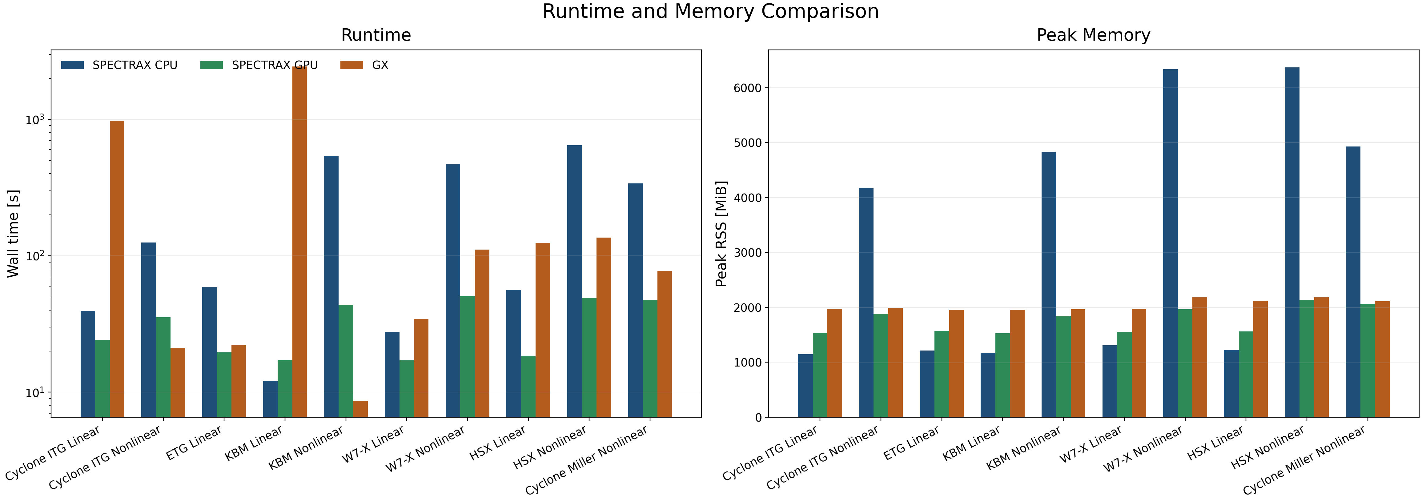
The runtime subplot uses a log scale because the wall times span roughly three orders of magnitude; the memory subplot stays linear because the peak-RSS spread is much narrower. The panel is regenerated from the tracked summary with:

python scripts/benchmarks/benchmark_runtime_memory.py \
  --summary-glob docs/_static/runtime_memory_summary_ship_refresh.json \
  --csv-out docs/_static/runtime_memory_results_ship_refresh.csv \
  --summary-out docs/_static/runtime_memory_summary_ship_refresh.json \
  --plot-out docs/_static/runtime_memory_benchmark.png

A PDF companion is emitted for manuscript workflows and is not tracked.

The panel reports cold wall time, which for the JAX backends includes startup and compilation. That is the right number for “how long does one run take” and the wrong one for “how fast is the kernel”, and it makes short nonlinear cases look worse than their throughput: in docs/_static/runtime_memory_results_ship_refresh.csv the GPU Cyclone nonlinear row is 35.33 s against 21.15 s for GX, and KBM nonlinear 43.74 s against 8.68 s. The runner overlays a warm second-run marker wherever a row has run_time_s; the shipped summary has none, so the panel shows cold times only. Warm throughput is what the prepared profiles above measure. For these short lanes the useful work is compile and startup reduction and executable reuse, which the persistent compilation cache addresses, rather than per-step kernel work alone.

Preconditioner policies

Preconditioner choices, with shape, finite-value, linked-boundary and shift-invert contracts covered by tests/unit/linear/test_linear.py and tests/unit/linear/test_linear.py:

• the implicit (backward-Euler GMRES) time integrator accepts diag (damping plus the curvature/grad-B diagonal), damping, pas (the PAS streaming line solve with diagonal damping and drifts), pas-coarse (line plus a kx-coarse additive correction), hermite-line (the tridiagonal Hermite streaming solve at fixed \(k_z\)), hermite-line-coarse, and identity;

• the shift-invert eigensolver accepts hermite-line and hermite-line-coarse, field-corrected and field-corrected-coarse, pr3-cm, damping and none. pr3-cm runs three Peaceman–Rachford double sweeps of the Hermite line solve with the z-mean drift against an exact z-local drift/mirror/field block, solved by block-Thomas in the Laguerre index plus Sherman–Morrison. It certifies on the shipped Cyclone deck, but its cost is set by applying the preconditioner rather than by iteration count, and it is not cheaper than the default adaptive eigensolver; Solvers gives the measured comparison and Numerics its structural preconditions.

Fresh runtime or iteration-count claims should be added through the tracked performance manifest and profiling tools, not through standalone probe scripts.

Parallel scaling

Parallel evidence lives in Parallelization policy; this section records only the boundary it draws. Production parallelization starts with independent work rather than nonlinear domain decomposition. gkx.ky_scan_batches and gkx.batch_map split k_y scans and quasilinear/UQ ensembles while preserving serial ordering, and the tracked large-run artifacts independent_ky_scan_scaling_large.json and quasilinear_uq_ensemble_scaling_large.json are the ones to cite. Sensitivity sweeps are covered by the same ordering/provenance utilities, but need their own scaling artifact before any speedup claim is promoted.

Whole-state nonlinear sharding is tracked in nonlinear_sharding_strong_scaling_large.json and gated by nonlinear_sharding_production_speedup_gate.json; its timing ratios are profiler evidence and not a production nonlinear speedup claim. The velocity-space linear-slice regime map is linear_rhs_parallel_slices_sweep.json. The earlier two-device linear scaling data in docs/_static/scaling_speedup_data.csv was measured on a Diffrax linear route GKX no longer ships; it is a historical record, replotted with python scripts/artifacts/plot_scaling_panels.py legacy-two-device (retired; Retired generators), not a reproducible artifact.

Communication-aware nonlinear domain decomposition remains diagnostic until the exact workload has identity, communication, transport-window, and matched profiler evidence for any nonlinear multi-GPU speedup claim. If a future optimization changes that conclusion, refresh the CPU and GPU artifacts before changing README or release-note wording; the boundary is mirrored in Features and Claim Scope.