Quasilinear Transport
GKX computes quasilinear transport diagnostics from a linear eigenstate or a late-time linear state. The linear diagnostic and the saturation model are kept separate:
linear weights are amplitude-normalized heat and particle fluxes computed with the same diagnostic kernels as runtime simulations;
saturation rules are named, serialized model assumptions that convert a linear mode into a trend-level saturated estimate;
calibrated absolute flux requires nonlinear training and holdout validation and cannot be inferred from an uncalibrated rule.
Status
The quasilinear layer is a scoped core-portfolio diagnostic and optimization-screening tool. It is not a runtime/TOML absolute-flux predictor, and the tracked calibration reports are not a calibrated absolute-flux claim.
One-constant saturation rules fail the held-out transport gate on the 12-case portfolio (2 training, 10 held-out nonlinear windows): held-out mean relative error 6.49 for positive-growth mixing length, 4.42 for the raw linear weight, 6.85 for absolute-growth mixing length, against a gate of 0.35.
The best reduced candidate,
spectral_envelope_ridge, reaches leave-one-geometry-out mean relative error 0.697 with interval coverage 11/12. It is not exposed as a runtime saturation law.On the declared 10-case core portfolio (Solovev and shaped-pressure external VMEC excluded as stress outliers), the same candidate passes the transport and coverage gate: mean relative error 0.280, held-out 0.275, maximum 0.575, coverage 10/10. The core rank-screening gate fails (Spearman 0.745 against 0.75).
The numbers come from docs/_static/quasilinear_saturation_rule_sweep.json,
docs/_static/quasilinear_candidate_uncertainty.json and the
core_portfolio_gate block of docs/_static/quasilinear_error_anatomy.json.
Literature anchors
The separation of linear weights from a saturation rule follows nonlinear tests of quasilinear transport [Waltz09], the QuaLiKiz derivation [Stephens21], profile-evolution use [Citrin17] and the review [Staebler24]. Parker et al. [Parker23] compare saturation rules as model assumptions rather than consequences of the linear solve. SAT3 [Dudding22] and SAT3-NN [Sar26] use spectrum-aware, database-calibrated saturation instead of one mixing-length constant. For stellarator optimization GKX uses quasilinear fluxes as research diagnostics and optimization proxies, following [Jorge24].
Configuration and outputs
Only the electrostatic channel is implemented; channels other than
"es" raise an error
(gkx.diagnostics.quasilinear_transport.normalize_quasilinear_channels).
[quasilinear]
enabled = true
mode = "weights"                 # or "saturated"
saturation_rule = "none"
amplitude_normalization = "phi_rms"
kperp_average = "phi_weighted"
csat = 1.0
gamma_floor = 0.0
include_stable_modes = false
channels = ["es"]
The diagnostic writes:
*.quasilinear.summary.json: growth rate, frequency, normalization,kperp_eff2, species weights and saturation metadata;*.quasilinear_species.csv: species-resolved heat and particle flux weights and, when requested, saturated estimates;*.quasilinear_spectrum.csv: one row perkyforgkx scanruns.
In the spectrum file ky is the requested scan coordinate (used for ordering
and plotting) and mode_ky is the signed grid mode the linear solve selected.
Keeping both stops negative-branch aliases from reordering linked-boundary or
imported-geometry spectra.
Running it
gkx run \
  --config examples/08_quasilinear/case_full.toml \
  --out tools_out/cyclone_quasilinear
or enable the diagnostic for another linear TOML from the command line:
gkx run \
  --config examples/01_linear_tokamak/case_full.toml \
  --quasilinear \
  --ql-mode saturated \
  --ql-saturation-rule mixing_length \
  --ql-normalization phi_rms \
  --ql-csat 1.0 \
  --out tools_out/cyclone_quasilinear
For a ky spectrum use gkx scan. --workers runs the per-ky
solves in parallel and keeps the serial ordering of the spectrum:
gkx scan \
  --config examples/08_quasilinear/case_full.toml \
  --ky-values 0.1,0.2,0.3,0.4 \
  --quasilinear \
  --workers 2 \
  --out tools_out/cyclone_quasilinear_scan

# retired generator; restore it first: git show f005418bf575:scripts/artifacts/plot_quasilinear_diagnostics.py > scripts/artifacts/plot_quasilinear_diagnostics.py
python scripts/artifacts/plot_quasilinear_diagnostics.py spectrum \
  --spectrum tools_out/cyclone_quasilinear_scan.quasilinear_spectrum.csv \
  --out tools_out/quasilinear_cyclone_spectrum.png
The serial/worker identity gate for this path
(docs/_static/quasilinear_runtime_parallel_gate.json) checks ordered
identity of the linear heat-flux weight and the saturated estimate; its timing
fields are engineering metadata, not a speedup claim:
JAX_ENABLE_X64=1 python scripts/artifacts/generate_parallel_identity_gate.py quasilinear-runtime \
  --workers 2 --ky 0.1 0.2 \
  --out-prefix docs/_static/quasilinear_runtime_parallel_gate
The Miller companion spectrum uses ky values resolved by the nonlinear
run’s Ny = 64 grid:
gkx scan \
  --config benchmarks/cases/cyclone_miller_quasilinear.toml \
  --ky-values 0.1,0.2,0.3,0.4,0.5 \
  --quasilinear \
  --out docs/_static/quasilinear_cyclone_miller_spectrum_scan
Model
Linear eigenproblem
For a fixed flux tube and perpendicular mode the linear runtime solves the matrix-free system
where G is the Hermite-Laguerre gyrocenter moment state, v_j a right
eigenvector, gamma the growth rate and omega the mode frequency
reported by the executable. The operator is assembled in
gkx.terms.assembly from the term modules under gkx.terms.
Field solve and linear weights
Fields are reconstructed from G with
gkx.terms.assembly.compute_fields_cached. The quasilinear diagnostic uses
phi and sets A_parallel = B_parallel = 0. The electrostatic heat-flux
weight contracts the radial \(E\times B\) velocity with the
Hermite-Laguerre pressure moment:
J_{ls} are the Laguerre gyroaverage coefficients of species s and
W_k includes the positive-ky Hermitian factor, the dealias mask, the
flux-surface Jacobian and grad rho weight, species density and temperature
factors, and the diagnostic flux scale. The particle-flux weight uses the
density moment,
and is zero for one-ion adiabatic-electron cases. The kernels are
gkx.diagnostics.heat_flux_species(),
gkx.diagnostics.particle_flux_species() and
_heat_flux_channel_contrib_species in gkx.operators.moments.
Amplitude normalization and effective scale
The averages use the runtime spectral and flux-tube volume weights, so the weights are invariant under eigenfunction phase rotation and amplitude rescaling. The default normalization is
with the weights of
gkx.diagnostics.quasilinear_transport.spectral_phi_weights(), whose
(k_y, k_x) factor is gkx.core_ky_layout.hermitian_mode_weights()
(see Numerics).
amplitude_normalization accepts:
phi_rms: weighted|phi|^2average (default);phi_midplane: maximum midplane|phi|^2;field_energy: electrostatic field energy.
Saturation rules
saturation_rule sets the squared amplitude \(A_k^2\); the saturated
fluxes are \(Q_{s,k}^{(\mathrm{sat})} = A_k^2 \widehat{Q}_{s,k}\) and
\(\Gamma_{s,k}^{(\mathrm{sat})} = A_k^2 \widehat{\Gamma}_{s,k}\).
Rule |
\(A_k^2\) |
Use |
|---|---|---|
|
not computed |
linear weights only |
|
\(C_{\rm sat}\max(\gamma_k-\gamma_{\rm floor},0)/k_{\perp,{\rm eff},k}^2\) |
baseline rule |
|
same as |
named alias kept for input compatibility |
|
\(C_{\rm sat}\) |
tests whether the weight spectrum alone transfers across geometries |
|
\(C_{\rm sat}|\gamma_k|/k_{\perp,{\rm eff},k}^2\) |
stress test that gives stable branches nonzero intensity |
include_stable_modes = true drops the max(., 0) clamp. A rule returns
zero when kperp_eff2 is non-positive or non-finite. These rules are
baselines for software validation and sensitivity studies; none is a
predictive absolute-flux model.
gkx.diagnostics.quasilinear_transport.quasilinear_feature_objective exposes
the same rules on feature vectors [gamma, kperp_eff2, flux_weight]; the unit
tests check its Jacobians against central finite differences.
Implementation map
Layer |
Source |
Responsibility |
|---|---|---|
Quasilinear weights |
|
|
Diagnostic kernels |
|
heat, particle and field-energy contractions shared by linear and nonlinear paths |
Runtime plumbing |
single-run and scan execution, command-line overrides, JSON/CSV writing |
|
Input schema |
|
|
Calibration reports |
|
train/holdout/audit schemas, spectrum integration, nonlinear-window ingestion, scale fitting and scoring |
Plotting tools |
|
spectrum, shape-gate and calibration figures |
Differentiability gates |
finite-difference checks, dense operator fixtures and implicit isolated-eigenpair sensitivities |
Algorithm
One linear mode:
build grid, geometry, species and linear cache
solve the eigenproblem or fit the late-time linear state
reconstruct phi; compute kperp_eff2 from |phi|^2 weights
contract heat and particle fluxes with the runtime diagnostic kernels
divide by the amplitude normalization; optionally apply a saturation rule
write summary JSON and species CSV
A ky scan repeats this per requested ky, selects the closest grid mode,
stores ky and mode_ky, and writes *.scan.csv and
*.quasilinear_spectrum.csv.
Calibration against nonlinear windows:
load a nonlinear diagnostic CSV or NetCDF over a declared time window
compute late-window convergence metadata after transient removal
require finite mean, running-mean drift, block-bootstrap SEM and provenance
integrate the linear quasilinear spectrum
create train, holdout or audit points
optionally fit one multiplicative scale on train points only
score holdouts against the mean-relative-error and window gates
Differentiability
Production linear solves are matrix-free. Dense matrices are built only in
small validation fixtures by
gkx.objectives.autodiff_validation.explicit_complex_operator_matrix().
Eigenvalue sensitivities use JAX derivatives of the matrix entries and the
isolated-branch relation
where v and w are right and left eigenvectors. Eigenfunction-dependent
observables use the implicit perturbation system
with gauge w^\dagger \partial_i v = 0, which makes the derivative unique for
phase-invariant observables. jnp.linalg.eig does not differentiate
non-Hermitian eigenvectors unless the caller opts in through
lax_linalg.eig(..., enable_eigvec_derivs=True) (jax >= 0.10.1); the
implicit left/right path is the validation route for quasilinear observables.
examples/08_quasilinear/implicit_sensitivity.py applies it to
a small Cyclone linear-RHS fixture. The differentiated observable is
\([\gamma, \omega, k_{\perp,\mathrm{eff}}^2, \widehat{Q}_i,
Q_i^{(\mathrm{ML})}]\), where \(Q_i^{(\mathrm{ML})}\) is the uncalibrated
mixing-length heat-flux proxy, with respect to [a/L_n, a/L_Ti]. Against
central finite differences that follow the nearest isolated branch, the tracked
artifact docs/_static/quasilinear_implicit_sensitivity.json records maximum
relative derivative error 1.2e-2 at eigenvalue gap 0.24.
python examples/08_quasilinear/implicit_sensitivity.py
Tests
The fast suite covers:
TOML and command-line plumbing for
[quasilinear];phase and amplitude invariance of the linear weights;
rejection of electromagnetic channels;
summary and species artifact serialization, and ordered worker scans;
AD-versus-finite-difference checks of
quasilinear_feature_objectiveand of isolated-eigenvalue and implicit eigenpair sensitivities on small dense GKX linear-RHS fixtures;the promotion guardrail described below.
Calibration reports
Calibration artifacts use scripts.checks._gates.quasilinear_calibration, so
train, holdout and audit points share one schema. A report is promoted to
calibrated_absolute_flux only when it has at least one training point, at
least one holdout, passed finite late-window convergence metadata for every
holdout, and a passed holdout mean-relative-error gate. Otherwise it is demoted
to calibration_dataset or training_or_audit_only.
The one-constant fit is
where \(q_j^{\rm raw}\) is the unscaled spectrum sum and \(Q_j^{\rm NL}\) the nonlinear window mean. The gate is
Window metadata comes from scripts.checks._gates.transport_windows or
scripts/checks/check_nonlinear_transport_gates.py convergence and records the
transient cutoff, late-window mean and standard deviation, running-mean drift,
block-bootstrap SEM, sample counts and source provenance. Replicated windows are
combined with scripts.checks._gates.transport_windows.nonlinear_window_ensemble_report
(command line: check_nonlinear_transport_gates.py ensemble), which requires
every input window to be promotion-ready and checks the relative spread of the
late-window means and the combined SEM. check_nonlinear_transport_gates.py
matched-windows compares two passed windows, for example with and without an
intervention, and reports the relative reduction with its quadrature-SEM
separation.
The report builder rejects points whose rule differs from the report’s
saturation_rule, non-finite predictions or window means, negative window
standard deviations, missing spectrum columns, all-non-finite samples and
non-positive delta_ky.
calibration_point_from_nonlinear_window_summary converts a nonlinear window
summary into a calibration point. CSV inputs use the t column and the
selected heat-flux column (usually heat_flux). NetCDF inputs use
Grids/time and map heat_flux to Diagnostics/HeatFlux_st and
heat_flux_es/heat_flux_apar/heat_flux_bpar to the matching
Diagnostics/HeatFlux*_st variables. Species are summed by default; pass
--species-index to the report builder for an ion-only or electron-only
target. The window is the summary’s tmin/tmax when present, otherwise
the full finite range.
python scripts/artifacts/plot_quasilinear_calibration.py report \
  --spectrum docs/_static/quasilinear_cyclone_spectrum_scan.quasilinear_spectrum.csv \
  --nonlinear-summary docs/_static/nonlinear_cyclone_gate_summary.json \
  --split audit \
  --case cyclone_long_window \
  --geometry cyclone \
  --electron-model adiabatic \
  --saturation-rule mixing_length \
  --out docs/_static/quasilinear_cyclone_calibration_audit_report.json

python scripts/artifacts/plot_quasilinear_calibration.py \
  --report docs/_static/quasilinear_cyclone_calibration_audit_report.json \
  --out tools_out/quasilinear_cyclone_calibration_audit.png
With C_sat = 1 the mixing-length rule underpredicts the Cyclone nonlinear
heat flux by orders of magnitude, so this audit report stays
training_or_audit_only.
Guardrails
scripts/checks/check_quasilinear_promotion_guardrails.py calibration-inputs
matches each train/holdout point’s nonlinear_artifact to tracked, passed
nonlinear gate metadata, so an exploratory or non-converged pilot cannot enter
calibration. scripts/checks/check_quasilinear_promotion_guardrails.py
without a subcommand audits the calibration and model-selection JSON reports
(finite window statistics, train/holdout provenance, passed held-out gates
before calibrated_absolute_flux), scans documentation for scope markers and
positive absolute-flux wording, and checks that each quasilinear figure in the
manuscript index has a JSON sidecar and a non-absolute claim level. Its output
is docs/_static/quasilinear_promotion_guardrails.json.
Calibration portfolio
The combined report docs/_static/quasilinear_stellarator_train_holdout_report.json
fits on two training windows and scores ten held-out windows, all adiabatic
electron, electrostatic ITG. \(\langle Q_i\rangle\) is the admitted
nonlinear window mean in gyro-Bohm units.
Case |
Split |
Admission |
\(\langle Q_i\rangle\) |
|---|---|---|---|
Cyclone s-alpha |
train |
long-window nonlinear gate |
6.67 |
ITERModel external VMEC |
train |
|
22.05 |
Cyclone Miller |
holdout |
long-window nonlinear gate |
4.26 |
HSX (QHS deck) |
holdout |
|
5.09 |
W7-X |
holdout |
|
5.38 |
D-shaped external VMEC |
holdout |
|
18.48 |
Up-down asymmetric external VMEC |
holdout |
|
7.76 |
Circular external VMEC |
holdout |
|
19.43 |
CTH-like external VMEC |
holdout |
|
9.60 |
Shaped-pressure external VMEC |
holdout |
|
7.16 |
QP |
holdout |
replicated |
16.40 |
Solovev external VMEC |
holdout |
replicated |
1.41 |
CTH-like and shaped-pressure are admitted only under coarse-grid exclusion:
their full n48/n64/n80 ladders fail (shaped-pressure grid shift 0.469
against 0.15), so neither is a full-ladder convergence claim. The admission
sidecars are
docs/_static/external_vmec_cth_like_modified_high_grid_admission_gate.json
and
docs/_static/external_vmec_shaped_tokamak_pressure_dt0p04_high_grid_admission_gate.json;
the ensemble gates are named in each point’s nonlinear_artifact.
Excluded windows and the reason for each are listed under
excluded_candidates in docs/_static/quasilinear_holdout_gap_report.json.
They include:
KBM: electromagnetic, while the quasilinear channels are electrostatic;
nfp4 QH external VMEC: grid shifts 0.523/0.480 (
n32/n48) and 0.630/0.704 (n48/n64) on the common/least-trending windows, above 0.15;a same-family ITERModel
t = 450audit: reproducibility evidence for the training reference, not an independent holdout.
The QI seed equilibrium (quasilinear_vmec_qi_seed_linear_spectrum_scan)
peaks at \(\gamma \approx 3.8\times10^{-3}\) near ky = 0.143, below the
0.02 nonlinear-launch threshold of scripts/artifacts/build_qi_branch_refinement_gate.py (retired; Retired generators),
so no nonlinear window exists for it.
Results
Test |
Result |
Artifact |
|---|---|---|
One-constant transfer, Cyclone to Cyclone Miller |
fitted |
|
One-constant transfer, 12 cases |
held-out mean relative error 6.49; worst holdout Solovev (predicted 53.2, observed 1.41) |
|
Saturation-rule sweep |
linear weight 4.42, mixing length 6.49, absolute growth 6.85, training-mean null 1.80; no rule accepted |
|
Shape-aware power law |
leave-one-geometry-out error 0.725 against linear weight 0.624 and
training-mean null 0.170; |
|
Candidate uncertainty |
|
|
Ridge-penalty sweep |
best |
|
Rank screening |
|
|
Residual anatomy |
external axisymmetric VMEC cases carry 83% of the
|
|
Model selection |
blockers |
|
All artifacts are under docs/_static/. Every model-development report
carries an input_validation block built from the nonlinear summary gates, so
it can only be regenerated from windows that passed those gates.
HSX and W7-X
Every scanned HSX and W7-X branch in the tracked short electrostatic
adiabatic-electron spectra is stable, so with gamma_floor = 0 the
mixing-length estimate is zero while the nonlinear windows are finite (relative
error one by construction). The raw linear-weight fit overpredicts both by
roughly a factor of four; spectral_envelope_ridge is closer
(docs/_static/quasilinear_stellarator_usefulness.json).
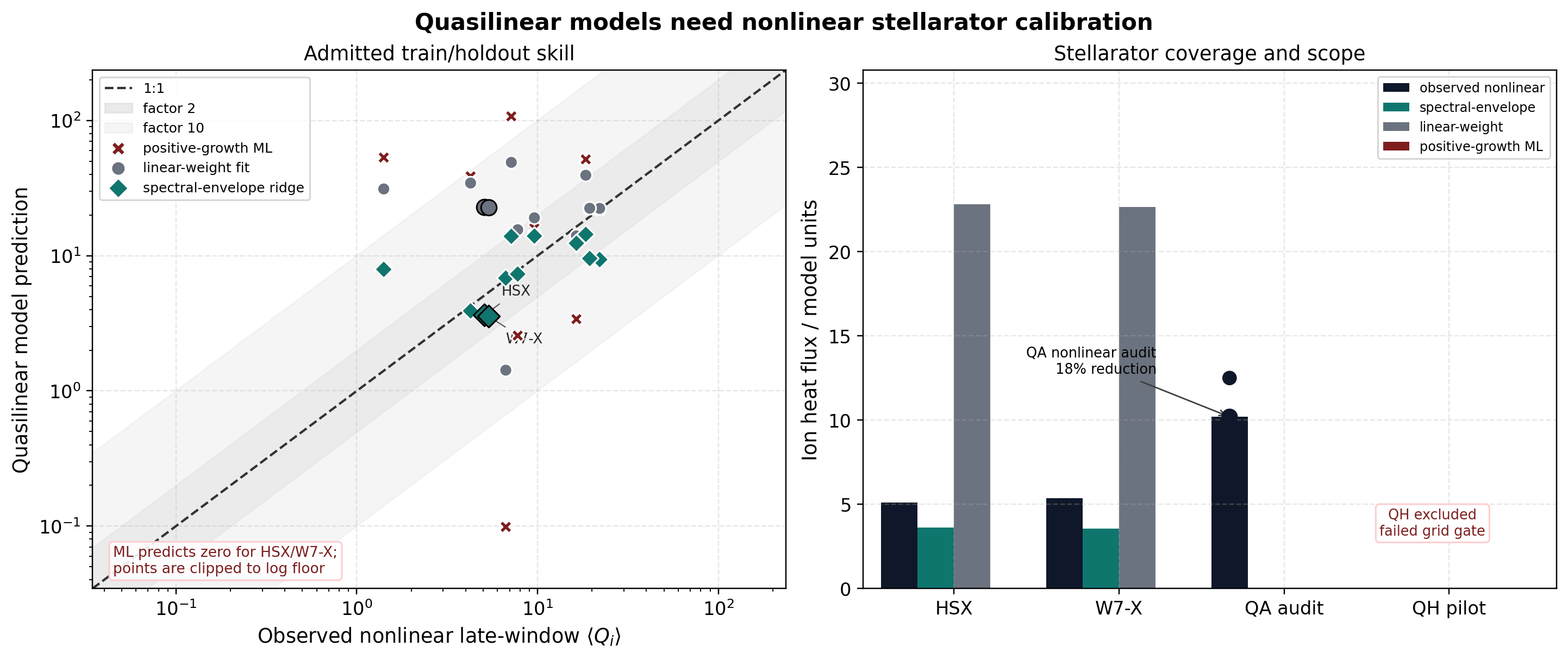
Stellarator saturated states involve subdominant and stable eigenmodes [Pueschel16], energy transfer to damped modes [Hegna18] and zonal-flow dynamics [Tiwari25], and linear growth rates are a weak proxy for saturated heat flux across quasi-symmetric configurations [McKinney19]. In GKX, quasilinear metrics are used for screening, differentiable-optimization research and model development, not for absolute stellarator heat flux.
The HSX input is the Nuhrenberg-Zille QHS deck generated by vmex; the W7-X
command uses the shipped QI deck. For the benchmark equilibria, point
[geometry].vmec_file at the machine-specific WOUT, which is not in Git.
cd examples/vmec
vmex input.NuhrenbergZille_1988_QHS
vmex input.nfp3_QI_fixed_resolution_final
cd ../..
gkx scan \
  --config examples/02_linear_stellarator/case_full.toml \
  --ky-values 0.047619047619047616,0.09523809523809523,0.14285714285714285,0.19047619047619047,0.23809523809523808,0.2857142857142857 \
  --Nl 4 --Nm 8 --solver time --dt 0.005 --steps 400 \
  --quasilinear \
  --out docs/_static/quasilinear_hsx_spectrum_scan \
  --no-progress
gkx scan \
  --config benchmarks/cases/w7x_linear_quasilinear_vmec.toml \
  --ky-values 0.047619047619047616,0.09523809523809523,0.14285714285714285,0.19047619047619047,0.23809523809523808,0.2857142857142857 \
  --Nl 4 --Nm 8 --solver time --dt 0.005 --steps 400 \
  --quasilinear \
  --out docs/_static/quasilinear_w7x_spectrum_scan \
  --no-progress
Each holdout is added to the Cyclone/Miller report with, for W7-X:
python scripts/artifacts/plot_quasilinear_calibration.py report \
  --points docs/_static/quasilinear_cyclone_miller_train_holdout_points.json \
  --spectrum docs/_static/quasilinear_w7x_spectrum_scan.quasilinear_spectrum.csv \
  --nonlinear-summary docs/_static/nonlinear_w7x_gate_summary.json \
  --split holdout \
  --case w7x_nonlinear_window \
  --geometry w7x \
  --electron-model adiabatic \
  --fit-train-scale \
  --out docs/_static/quasilinear_w7x_train_holdout_report.json
Spectrum-shape gates
A shape gate compares only the normalized ky distribution of the linear
heat-flux weight with the resolved nonlinear Diagnostics/HeatFlux_kyst
spectrum; it does not test the absolute level. Pass criteria are total
variation TV <= 0.2 and cosine similarity >= 0.95.
Case |
TV |
cosine |
Result |
|---|---|---|---|
W7-X |
0.056 |
0.992 |
pass |
HSX |
0.11 |
0.97 |
pass |
Cyclone Miller |
0.094 |
0.983 |
pass |
Cyclone s-alpha (long window) |
0.215 |
0.896 |
fail; mismatch in the low- and high- |
The values are in docs/_static/quasilinear_<case>_spectrum_shape_gate.json.
KBM has no shape gate because its nonlinear lane is electromagnetic.
# retired generator; restore it first: git show f005418bf575:scripts/artifacts/plot_quasilinear_diagnostics.py > scripts/artifacts/plot_quasilinear_diagnostics.py
python scripts/artifacts/plot_quasilinear_diagnostics.py shape-gate \
  --spectrum docs/_static/quasilinear_hsx_spectrum_scan.quasilinear_spectrum.csv \
  --nonlinear tools_out/final_nonlinear_audit/hsx_nonlinear_t50.out.nc \
  --out tools_out/quasilinear_hsx_spectrum_shape_gate.png \
  --ql-column heat_flux_weight_total \
  --nonlinear-variable Diagnostics/HeatFlux_kyst \
  --time-max 49.2 \
  --tv-gate 0.2 \
  --cosine-gate 0.95
The nonlinear NetCDF inputs are local run outputs and are not tracked.
Convergence evidence
Admission follows the practice of nonlinear benchmark papers: a saturated heat-flux window is used only if it is robust to resolution and window choice [Dimits00] [GX] [GonzalezJerez22]. The 0.15 grid-shift threshold is of the order of the heat-flux convergence tolerances reported for Laguerre-Hermite calculations in [GX]. Stellarator flux-tube domain choices change results [Sanchez21], which is why external-VMEC cases sit behind explicit gates. Turbulent flux traces are autocorrelated and need uncertainty and stopping checks [Oberparleiter16], low velocity resolution can move the saturated heat flux [Hoffmann23], and W7-X heat-flux time series show the same statistical structure [Papadopoulos23].