Numerics
This page describes how GKX discretizes and integrates the operator stated in Operators And Terms, the defaults a run takes when a deck leaves a choice open, and the numerical checks behind them. Solver selection and eigenvalue certification are covered in Solvers.
Spectral discretization
Perpendicular coordinates are Fourier modes on a uniform grid in \(x\) and \(y\); the parallel coordinate is resolved in real space along the field line, and differentiated spectrally. Velocity space uses a Hermite-Laguerre basis. The state layout for one species is
(N_l, N_m, N_y, N_x, N_z).
JAX execution model
jax.jit stages the integrators and jax.lax.scan drives the time loop.
Implicit time steps and shift-invert inner solves use solvax.gmres
(right-preconditioned FGMRES); nonlinear IMEX reverse mode wraps it in
solvax.linear_solve, whose implicit-function VJP solves the transposed
system instead of differentiating the iterations. The Hermite line solve uses
solvax.tridiagonal_solve. solvax.chunked_jacfwd bounds memory for
geometry Jacobians; chunking changes batching, not the columns. Generic
algebra lives in SOLVAX (the floor is declared once, in pyproject.toml);
state layout, linked-boundary assembly, preconditioner coefficients, branch
tracking, transport windows and physics gates stay in GKX. Module names are in
Design and Code Map.
Time integration algorithms
Linear integrators (gkx.solvers_linear_integrators.integrate_linear())
share the cached operator data of
gkx.operators.linear.cache_builder.build_linear_cache():
Explicit
rk2,rk4,sspx3; CFL-controlled (integrate_linear_explicit), which recomputes the step from the linear max-frequency estimate (defaultsrk4,fixed_dt=False,cfl=0.9).Diagonal IMEX
imex(first order) andimex2: diagonal collision and hypercollision damping implicit, everything else explicit.Backward Euler + GMRES
implicit, with the physical preconditioner named inimplicit_preconditioner.
imex2 is the ARS(2,2,2) split.
For a diagonal non-negative damping \(D\) and explicit remainder \(E\),
with \(\gamma=1-1/\sqrt{2}\) and \(\delta=1-1/(2\gamma)\):
It is second order and L-stable for pure damping; with \(D=0\) its
stability polynomial is explicit midpoint’s. Nonlinear runs use an explicit
scheme (rk2, rk3, rk4, sspx3),
imex (linear operator implicit by GMRES, bracket explicit) or the opt-in
imex-ars3 (Resolution, Step and Solver Guidance). The CFL prefactor cfl_fac is 1.73 for
rk3/sspx3, 2.82 for rk4, 1.0 otherwise. Reverse derivatives of the
IMEX route use the converged-system implicit derivative.
What a first run gets
Defaults for a deck that leaves a choice open, each backed by a load-independent measurement (Measurements behind the defaults):
Eigen route:
auto, banded direct shift-invert where it fits, elseadaptive, the residual-certified propagator eigensolve (Solvers).Precision:
complex64. On01_linear_tokamak/case_full.tomlfloat32 gives \(\gamma = 0.09309106\) against float64’s \(0.09309117\) (1.2e-6 relative);JAX_ENABLE_X64=trueapplies the float64 certification gate (1e-9 against 1.19e-4) at about 17% more memory.Step: a deck that sets
[time] dtkeepsrk2at that step; a deck withoutdtgetsrk4with the CFL controller. Fixed-step linear paths warn whendtexceeds the CFL estimate.Resolution:
(Nl, Nm) = (12, 24)linear,(4, 8)nonlinear, a starting point and not a convergence statement.Nonlinear horizon: diagnosed runs stop at saturation, with
t_maxas the cap (Saturation stop policy).Unchanged: two-thirds dealiasing;
collisionsandhypercollisionsenabled as terms with per-speciesnu = 0; the persistent compilation cache on, so a second run skips compilation; the CPU FFT thread pool stays on (single-threaded measured 8–10% slower).
Measurements behind the defaults
Shipped Cyclone deck, float32, counting propagator applies, steps and right-hand-side evaluations rather than wall time.
default |
value |
accuracy |
|---|---|---|
|
40 |
residual 9.50e-01; 200 applies give 9.47e-01; neither certifies |
|
rk4, CFL-controlled |
-2.63e-04 relative to the certified eigensolve |
|
(12, 24) |
+0.400% of the tracked GX golden |
power_iters. At (4, 8), ky = 0.3 the power ladder stalls near a residual
of 6e-3 (5000 applies) against the 1.19e-4 gate, so no count certifies and 40
is chosen for cost. No shipped deck selects the power route, and with
certify=True it raises rather than return an uncertified pair.
Time pairing. The defaulted dt = 0.1 is 7.8x the CFL-stable 0.01281, so
fixed-step rk2 and rk4 overflow. With the controller, rk2, rk3 and rk4 agree
within 3e-4 and rk4 needs 29.1% fewer right-hand-side evaluations (11072
against 15612 for rk2), exactly \(4/(2.82\times2)\). A deck that chooses
dt keeps rk2, and every shipped deck sets dt.
Resolution. Certified eigensolves at ky = 0.3 against the GX golden
\(\gamma = 0.09302951\):
Nl |
Nm |
gamma |
rel. to golden |
|---|---|---|---|
8 |
24 |
0.09877566 |
+6.177% |
24 |
12 |
0.08893196 |
-4.405% |
12 |
24 |
0.09340143 |
+0.400% |
12 |
32 |
0.09263792 |
-0.421% |
16 |
32 |
0.09284505 |
-0.198% |
24 |
24 |
0.09368346 |
+0.703% |
16 |
48 |
0.09309106 |
+0.066% |
All rungs certify at the 1.19e-4 gate. The ladder is not monotone, so
(12, 24) is where this case lands at that cost, not an error bound for another
case. Parallel phase mixing needs Hermite resolution while the FLR response
needs enough Laguerre; a deck whose physics runs the other way, such as the
ETG decks at Nl = 24, Nm = 8, says so.
Saturation stop policy
A diagnosed nonlinear run with run_to = "saturation" (the default)
integrates in chunks and asks
gkx.diagnostics.saturation.saturation_stop_decision() after each whether
the heat-flux trace supports a mean. It stops when every gate passes, or at
t_max, without claiming saturation. Spin-up is removed up to the first
crossing of the trace’s own median. The window mean’s standard error uses the
Sokal integrated autocorrelation time \(\tau\):
\(\mathrm{SEM} = s/\sqrt{n_\mathrm{eff}}\),
\(n_\mathrm{eff} = \min(n,\; n\,\Delta t/(2\tau))\). All of these must hold:
Gate (reason recorded when it fails) |
Condition |
|---|---|
|
the autocorrelation crosses zero inside the window and \(\tau > \Delta t\) |
retained samples |
at least 256 after spin-up |
|
window span at least \(20\tau\) and |
|
\(\mathrm{SEM}/|\text{mean}| \le\) |
|
first- and second-half means agree within twice their combined SEM |
|
the same half-window test for |
|
\(|\text{mean}| > 10^{-9}\) |
These are finite-sample safeguards, not a sequential-confidence guarantee, and
are not qualified for irregular adaptive sampling. The decision and its
reasons are written under saturation in the summary JSON. A prepared
simulation (gkx.prepare) compiles a fixed length, so it refuses
run_to = "saturation" unless given steps=N.
Distributed state sharding
TimeConfig.state_sharding = "auto" (or "ky"/"kx") partitions the
packed nonlinear state over several JAX devices; with one device it is ignored.
"z" is rejected (the FFT-axis decomposition has not passed its identity
gate) and the sharded path refuses a non-default collision_operator. Active
multi-device CPU sharding is skipped on macOS because XLA CPU FFT layouts can
abort. A speedup claim needs its own identity, transport-window and profiler
gates.
Nonlinear FFT bracket
The \(E\times B\) term is pseudospectral. By default
(compressed_real_fft = true) gradients come from the N_y/2+1
non-negative-\(k_y\) spectrum, matching the reference layout and minimizing
memory traffic. Electromagnetic runs stack J0*phi, J0*apar and the
bpar correction into one FFT batch.
Limitation (#336). The "grid" Laguerre bracket advects with the node-space
\(J_0\phi\) and keeps the first Nl coefficients, while quasineutrality
uses the analytic \(J_\ell\). The retained energy is then conserved only to
about \(7\times10^{-8}\) of the bilinear scale at Nl = Nm = 4. Treat
it as a resolution diagnostic, converged in Nl (Mandell, Dorland &
Landreman 2018, section 4.1).
The ky layout contract
gkx.core_ky_layout owns every conversion between two layouts of the
ky axis. full is the two-sided fftfreq order with Nky = Ny; the
runtime evolves it. half is the non-negative rfftfreq rows,
Nyc = 1 + Ny // 2; GX, stella and GS2 evolve it, and GKX uses it for
restarts, NetCDF output, spectra and snapshots. A real field obeys
\(F(-k_y, -k_x, z) = F^{*}(k_y, k_x, z)\). Three rules:
Nycdoes not determineNy: widening takesny_fullexplicitly.Row 0, and row
Ny/2for evenNy, are self-conjugate: \(F(k_x) = F^{*}(-k_x)\) within the row. Storingky >= 0does not enforce it; operators that write those rows callsymmetrize_self_conjugate_rows.Reductions of quantities even in \(k_y\) use
ky_row_weights(2 on paired rows, 1 on self-conjugate rows), never a blanket factor of two, which over-counts the Nyquist row. A flux on that row vanishes for a real field, and two-thirds dealiasing zeroes it anyway.
[grid] ky_layout = "half" is the default; "full" is the opt-out. On
Cyclone at 24x24x24 to 64x64x24 the two layouts agree to 2e-16 (x64) and
2e-7 (float32) in the nonlinear diagnostics, with even and odd Nyc, with
state_sharding = "ky" on four forced CPU devices, and bitwise in the
heat-flux window value and gradient; "half" runs the window gradient in 0.68
(CPU) to 0.72 (GPU) of the two-sided time (Performance).
Equilibrium-flow shearing coordinates
A research path, not an input option.
gkx.operators.nonlinear.projection.advance_shearing_coordinates()
follows \(k_x^*(t) = k_x(0) - k_y\gamma_E t\). When the displacement
crosses half a radial cell the state moves to the nearest \(k_x\), the
sub-cell residual is kept in the wavenumber and the phase
\(\exp(i\,\delta k_x x)\) (the corrected remap of [McMillan19]), and
modes leaving the two-thirds band are zeroed. The remap is piecewise constant
with a stopped tangent; wavenumbers and phases stay differentiable between
remaps. Non-twist tubes are refused. There is no parallel-velocity-gradient
drive [Schekochihin12] [Ball19]. Shear is expected to decorrelate turbulence
once the shearing rate exceeds the instability rate [Biglari90] [Waltz95];
the gate below tests that. Integrators:
integrate_nonlinear_sheared (RK2, RK3, fixed-step IMEX) and
integrate_nonlinear_sheared_transport. Treatment effects are judged with
matched_nonlinear_transport_report, not by comparing two chaotic traces.
The response gate fails, so flow shear stays out of input files.
docs/_static/flow_shear_fixed_step_response_gate.json (Cyclone ITG,
64x64x24, Nl=4, Nm=8, dt = 0.02, window \(t = [240, 300]\)):
integrator |
\(\gamma_E = 0\) |
\(\gamma_E = 0.01\) |
windows pass |
|---|---|---|---|
GKX fixed-step IMEX |
15.451 ± 0.263 |
16.195 ± 0.160 |
no |
independent fixed-step RK4 |
11.715 ± 0.216 |
14.624 ± 0.141 |
yes |
Both increase the heat flux (4.82% and 24.82%) instead of the required 5% reduction at two combined SEMs, which rejects the weak-shear suppression claim. The coordinate, remap, operator and derivative identities are not rejected.
Parallel boundary and end damping
A linked (twist-and-shift) chain is a finite piece of the infinite ballooning line. Its spectral \(z\) derivative is periodic over the chain, so what streams out of one end would re-enter at the other. GKX absorbs it in a layer at each end of every non-zonal chain:
with \(L_w\) = damp_ends_widthfrac (0.125) of the chain. The damped
quantity is the non-adiabatic \(h\), as in GX.
Contract. \(\nu_{end}\) is a rate in \(v_{ti}/a\) units and the
same on every route: time integration (any step, fixed or adaptive), Krylov,
eigen, shift-invert and nonlinear. No timestep enters. [time]
damp_ends_rate sets it. The default is
that is, 30 e-folds per thermal transit of the fastest kinetic species across a
layer of one segment (\(L_z\) is the stored \(z\) extent). Each run
prints the rate it uses (end damping: rate ...). A deck that sets only the
legacy damp_ends_amp is refused.
Why a rate. GX applies damp_ends_amp/dt (before February 2023,
\(5 v_{max}/L\)). Read as a rate, \(A/\Delta t\) makes a timestep-free
eigenvalue depend on a step it does not have. GS2 [KRT95] and stella [BPL19]
need no absorber (upwinded implicit streaming sets \(h = 0\) for incoming
particles); GENE truncates the \(k_x\) connection and uses parallel
hyperdiffusion [PDJ10]. A Hermite basis does not separate \(v_\parallel\)
directions, so GKX keeps GX’s layer and fixes only its units.
A GX nonlinear run applies \(A/\Delta t\) at its own step, so matching it
means setting damp_ends_rate to \(A/\Delta t_{GX}\); the W7-X ETG
flux moves by a factor of two over that range (Nonlinear W7-X ETG against GX).
Measured sensitivity (ky 0.3; plan/research/2026-10-15-end-damping;
\(\gamma\) in deck units):
deck (Nl, Nm), route |
nperiod |
C = 3 |
C = 10 |
C = 30 |
C = 100 |
|---|---|---|---|---|---|
adiabatic Cyclone (8, 16), Krylov |
2 / 3 / 4 |
0.09825 / 0.09831 / 0.09831 |
0.09829 / 0.09831 / 0.09831 |
0.09831 / 0.09831 / 0.09831 |
0.09825 / 0.09831 / 0.09831 |
kinetic-electron Cyclone (8, 16), time |
2 |
0.16786 |
0.16792 |
0.16803 |
0.16807 |
KBM s-alpha (4, 8), sparse eigen |
2 / 3 |
0.2364 / 0.2382 |
0.2441 / 0.2497 |
0.2426 / 0.2502 |
0.2407 / 0.2499 |
Below \(C \approx 1\) the kinetic-electron and KBM rates are not converged
(KE \(\gamma\) = 1.59 at C = 0, 0.174 at C = 1). Kinetic electrons at
(8, 16) are not converged in domain length (nperiod 3 gives 0.288); that is a
resolution question, not an absorber one. At nperiod = 1 the layer is a
quarter of the line and the adiabatic rate keeps falling with C
(0.0923 at C = 10, 0.0817 at C = 300): use nperiod >= 2.
Explicit steps. \(\nu_{end}\) is explicit, so \(\nu_{end}\Delta t\)
must stay inside the scheme’s stability region. It is below 0.3 on the shipped
nperiod >= 2 linear decks; an nperiod = 1 KBM deck (rate 598)
blew up at \(\Delta t = 10^{-3}\) and runs at \(5\times10^{-4}\). The
CFL estimate does not yet include \(\nu_{end}\).
Checking a result. Rerun at damp_ends_rate 3x above and below the
printed rate and at nperiod + 1. A converged growth rate moves by less
than its quoted tolerance in all three.
De-aliasing and hyperdiffusion
Nonlinear brackets use the standard 2/3 de-alias mask, stored on the
spectral grid and applied inside the bracket. Perpendicular hyperdiffusion
(D_hyper, p_hyper_kperp and the hyperdiffusion term weight; see
Operators And Terms) is available as scale-selective damping and is off by
default. \(k_{\perp,\max}\) is taken from the full grid’s dealiased corner,
also when a linear run keeps only a subset of ky rows.
Linear solver options
Batched ``ky`` scans:
ky_batch>1integrates severalkyat once;fixed_batch_shape=Truepads the last batch to avoid recompiling.Implicit preconditioners (
implicit_preconditioner):"auto"/"diag"/"physics"/"block","damping","pas","pas-coarse","hermite-line","hermite-line-coarse","identity".Shift-invert preconditioners (
KrylovConfig.shift_preconditioner):"damping";"hermite-line"(FFT in \(z\) plus a tridiagonal Hermite solve of the diagonal-plus-streaming symbol, \(O(n)\));"field-corrected"(the line plus the exact field response by a Woodbury capacitance solve);"pr3-cm"(below)."auto"is"pr3-cm"with the inner FGMRES raised to restart 150 and maxiter 600 (Methods and Decisions).Acceptance: every shift-invert pair is checked against the matrix-free relative residual \(\lVert Av-\lambda v\rVert/\max(\lVert Av\rVert,|\lambda|\lVert v\rVert)\) with
shift_outer_residual_tol(1e-6); rejected pairs raise. The eigenvalue is refreshed as the physical Rayleigh quotient.Branch selection:
KrylovConfig.mode_family("cyclone","etg","kbm") andshift_selection;fallback_methoddefaults to"propagator". Retained-Ritz thick restarts, projected Jacobi–Davidson and reduced Schur complements were tried for interior KBM eigenpairs, all chose the wrong branch, and none is shipped.Reusable IMEX operators:
build_nonlinear_imex_operatorprebuilds the matrix-free operator forintegrate_nonlinear_imex_cached.
The inner solves are right-preconditioned FGMRES started from zero. On the
first right-hand side of the outer Arnoldi (Cyclone, (Nz, Nl, Nm) = (96, 4,
8), float64) three GMRES(20) cycles from zero leave relative residuals of
0.995 (hermite-line), 0.9995 (field-corrected), 0.86 (damping) and
0.299 (pr3-cm); only pr3-cm converges unrestarted (9.9e-5 in 252
iterations), so raise shift_restart and shift_maxiter together.
pr3-cm (solvers_linear_precond_pr3.py) splits the operator into two
halves, each invertible in closed form, and sweeps between them. The Hermite
line solve inverts streaming, hypercollisions and the z-mean of the drift.
The rest (exact \(\omega_d(z)\), mirror, drive, end damping, collisions,
local field response) is z-local: dense \((l, m)\) blocks per
(species, ky, kx, z). One Peaceman–Rachford double sweep costs one solve of
each and no operator application; pr3-cm is three sweeps from zero, with
\(\alpha = -\sqrt{s_1 d}\) unless shift_precond_alpha is set. The
z-local block is solved by block-Thomas elimination in the Laguerre index plus
a Sherman–Morrison correction for the rank-one field part
(solvax.block_thomas_factor_ops), 1.5x to 2.7x smaller than a dense-band
factor. If the block is not l-tridiagonal, shift_precond_block_solve =
"auto" falls back to the dense batched inverse and records why; the build
also checks that the non-streaming operator is z-local and refuses otherwise
(zonal rows under adiabatic electrons fail it).
Automatic solver and fit-signal selection
solver = "auto" (default) runs the time path and falls back to the Krylov
eigensolve when the fitted (gamma, omega) is non-finite or violates
require_positive. fit_signal = "auto" fits both the phi and density
traces with the same windowing rules and keeps the higher score. Set
solver = "time", "explicit_time" or "krylov" and fit_signal =
"phi" or "density" to override.
Custom collision operators
Shipped models and the Python protocol are in Operators And Terms. A custom
operator is any JAX-compatible object with apply(context), passed as
collision_operator= to linear_rhs, linear_rhs_cached,
integrate_linear or nonlinear_rhs_cached. It runs on serial explicit and
IMEX linear integration and serial explicit nonlinear integration; implicit
linear solves, nonlinear IMEX, sheared IMEX and decomposed integration refuse
it. The finite-Larmor-radius coefficients are cancellation-sensitive, so they
are generated offline in multiple precision with their provenance and loaded as
compact arrays. Frei, Hoffmann & Ricci write the Bessel argument as
\(B=k_\perp\sqrt{2\tau}\); the runtime interpolates at \(B=\sqrt{2b}\).
Evidence files are docs/_static/collision_*.json.
Landau damping against the exact kinetic roots
The slab ion-acoustic dispersion relation with adiabatic electrons at \(k_\perp \to 0\),
with \(Z\) the plasma dispersion function (scipy.special.wofz), has no
free parameters. test_landau_root_recovered_by_collisional_extrapolation
evolves the production operator at \(N_m = 64\) and requires the
\(\nu \to 0\) extrapolation within 1% in \(\gamma\) and 0.5% in
\(\omega\) of the root, at \(T_e/T_i = 1\) and 10.
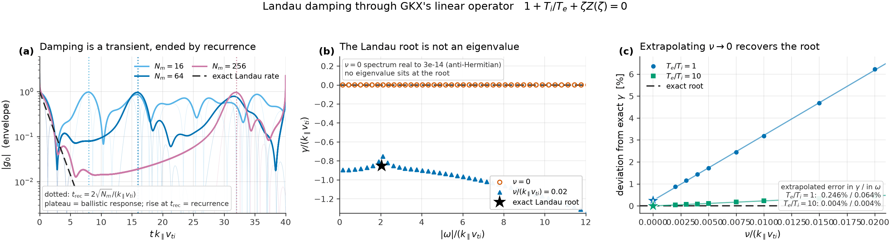
Produced by linear_rhs_cached; panel (b) eigen-decomposes the same
operator.
Four traps give plausible but wrong numbers (all gated in
tests/validation/physics_gates/test_collision_physics.py):
A collisionless truncated Hermite system cannot Landau damp: free streaming is anti-Hermitian, so the spectrum is real (\(\max|\mathrm{Re}\,\lambda| < 10^{-11}\)) and any fitted rate is a transient that ends at recurrence.
The Landau root is a pole of the continued response, not an eigenvalue. Add collisions, measure the decay at several small \(\nu\), extrapolate.
A density perturbation with no flow is a standing wave; fit \(A e^{\gamma t}\cos(\omega t + \phi)\), not an unwrapped phase.
tau_eis \(T_i/T_e\); the reciprocal is invisible at \(T_e=T_i\). GKX normalizes to \(v_{ti}=\sqrt{T/m}\), not \(\sqrt{2T/m}\).
Hermite closure and recurrence
Terminating the ladder with \(G_{M+1} = 0\) is a reflecting boundary: free energy returns to the low moments as recurrence at \(t_{\mathrm{rec}} \simeq 2\sqrt{M}/(k_\parallel v_{th})\). Because that grows only as \(\sqrt{M}\), the end of the ladder must absorb. GKX has two treatments.
Hypercollisions (default, [physics] hypercollisions = true) damp a band
of high moments with the \(|k_z|\)-scaled branch
\(\propto \nu_{hyper,m}|k_z|(m/M)^{p_m}\) (nu_hyper_m, p_hyper_m;
Operators And Terms).
Reflectionless closure (opt-in per species with [[species]]
hermite_closure = "reflectionless", LinearParams.closure; in the Python
streaming kernel hermite_closure="reflectionless") applies the
outgoing-wave condition of
Kanekar et al., J. Plasma Phys. 81, 305810104 (2015), Eq. (4.36):
a single sink \(-R_{M+1}\sqrt{M+1}\,v_{th}|k_\parallel|\,G_M\) on the last
moment. \(R_{M+1} \to 1 - 1/(4M)\), so the absorption becomes exact with
resolution; \(R_{M+1} > 0\) makes it a positive-definite energy sink; and it
touches only \(m = M\). At \(M = 2\) it reduces to the Hammett-Perkins
three-pole coefficient 0.921318. The test
test_absorbing_closures_beat_truncation_on_both_metrics requires each
treatment to cut the revived \(|g_0|\) below a tenth of truncation’s and
to keep the pre-recurrence error below 0.1, since suppression alone rewards any
strong damping. It carries no free parameter but is not a drop-in replacement
for a tuned hypercollision.
For a species with hermite_closure = "reflectionless" the sink replaces that
species’ \(|k_z|\) hypercollision band; it reuses the linked parallel
transform of that branch (no extra FFT) and appears in the explicit, implicit
and Hermite-windowed routes. It acts only where [physics] hypercollisions
is on. Other species, and the constant Laguerre branch and collision operator
of the closed species, are untouched; with the key omitted the right-hand side
is bitwise the one without the closure. The mixed species-Hermite electrostatic
route refuses it.
Measured effect. Dannert-Jenko trapped-electron mode (Miller \(q=1.4\),
\(\hat s=0.8\), \(T_e/T_i=3\), \(R/L_n=3\), \(R/L_{Te}=6\),
\(m_i/m_e=1836\), \(\beta_e=10^{-3}\), \(A_\parallel\),
\(N_l=8\), rk4, float64). Linear growth rate, hypercollision / closure,
against GS2:
\(k_y\rho_s\) |
|
|
|
|
GS2 |
|---|---|---|---|---|---|
0.2 |
0.349 / 0.388 |
0.468 / 0.487 |
0.531 / 0.537 |
0.601 / 0.613 |
0.675 |
0.3 |
0.624 / 0.661 |
0.786 / 0.806 |
0.855 / 0.865 |
0.938 / 0.949 |
1.005 |
0.5 |
0.991 / 1.028 |
1.203 / 1.229 |
1.282 / 1.298 |
1.367 / 1.378 |
1.402 |
The closure raises \(\gamma\) by 4 to 11 % at Nm 16 and by 1 to 2 % at
Nm \(\ge\) 48; at \(k_y\rho_s = 0.3\), Nm 192 gives 0.969 /
0.974. The frequency does not move (-0.922 / -0.923 at Nm 96), and the
\(\gamma\) deficit against GS2 at Nm 48 is 21/15/9 % with hypercollisions
and 20/14/7 % with the closure. Electron-temperature-gradient mode (GS2
\(k_y=10\), 3.988 / -6.212, \(N_l=24\)): Nm 32 3.988 / -6.227 against
3.986 / -6.229, Nm 16 4.022 / -6.200 against 4.028 / -6.202, so no
degradation where hypercollisions already converge. The explicit step bound is
unchanged: the Arnoldi radius of streaming, fields and the Hermite damping is
4887 / 10157 / 15009 (hypercollisions) and 5523 / 10717 / 15708 (closure) at
Nm 16 / 48 / 96, equal to streaming alone within 1 %, and the wall time at
Nm 48 is 181 s against 182 s.
Nonlinear check. The same trapped-electron case as a small nonlinear box
(\(8\times8\times32\), \(N_l=4\), random initial phases, rk4,
electromagnetic, same seed for every row), once with each closure on the
electrons. The effective growth rate of \(W_\phi\) before saturation is
0.95 to 0.97 at Nm 16 with hypercollisions, 1.02 to 1.03 with the closure
and 1.40 to 1.41 at Nm 48 (1.44 with the closure): the closure moves the
nonlinear growth by the same few percent as the linear rate, and both Nm 16
values are far below Nm 48.
After the first burst, \(t = 18\) to 30, the mean electron heat flux is
135 \(\pm\) 7 (hypercollisions) and 176 \(\pm\) 6 (closure) at Nm 16,
and 248 \(\pm\) 36 and 371 \(\pm\) 103 at Nm 32 (GKX units;
\(\pm\) is the spread of four time blocks; one seed, one box). The flux
rises with Nm and the closure moves it the same way, recovering about a
third of the Nm 16 to 32 step at Nm 16, but it is higher than the
hypercollision value at both Nm (+31 % and +50 %, the second within the
scatter) and is not shown to converge faster. All runs are stable and finite.
The saturated flux depends on the closure by more than the linear rate does, so
a switch changes pinned nonlinear baselines.
When to use it. It is a better truncation than the hypercollision band at the
same Nm, but a modest one: it does not remove the Hermite resolution error.
Use it for kinetic electrons when Nm is limited by cost and the
trapped-electron or ETG growth rate matters to a few percent, and compare it
with the default at two Nm before trusting either. Keep the default for
ions, for any species at Nm \(\ge\) 48 (the gain is 1 to 2 %, below
what a pinned baseline tolerates), and wherever a reference deck sets
hypercollisions deliberately. It is not on by default for kinetic electrons:
at Nm 16 the growth rate is still 27 to 43 % below GS2 with it (29 to
48 % without), and the remainder, 2 to 9 % at Nm 96, is resolution of the
trapped-passing structure (Nm 192 still moves). The closure costs nothing
extra but cannot be tuned: a deck that needs more damping of the top moments
has to keep the hypercollision band.
Operator assembly
Equations are in Operators And Terms. LinearTerms toggles convert to one
TermConfig (linear_terms_to_term_config), and
gkx.terms.assemble_rhs_cached sums the per-term kernels; the same RHS serves
the linear integrators, Krylov applications and nonlinear IMEX solves.
LinearParams.rho_star scales the perpendicular wavenumbers in the drift and
drive terms without changing the FFT spacing.
Nodal magnetic-moment grid
[run] mu_vperp_max (LinearParams.mu_vperp_max) replaces the Laguerre
expansion in \(\mu B\) by values at the nodes of a quadrature rule in the
fixed variable \(\hat\mu=\mu B_0\); Nl is then the number of nodes.
Unset keeps the Laguerre path, bitwise unchanged. The construction follows the
v2 representation of GX (Hermite spectral, \(\hat\mu\) nodal; GX docs/Numerics.rst,
“V2: Hermite plus nodal magnetic moment”) on the Hermite-Laguerre formulation of
Mandell, Dorland and Landreman, J. Plasma Phys. 84, 905840108 (2018).
Quadrature
Let \(\{\hat\mu_j,w_j\}_{j=1}^{n}\) satisfy
The \(\hat\mu_j\) are the eigenvalues of the Jacobi matrix of the monic
polynomials orthogonal for \(e^{-\hat\mu}\) on \([0,X]\), and
\(w_j=m_0 v_{0j}^2\) with \(m_0=1-e^{-X}\) and \(v_{0j}\) the first
component of the eigenvector (Golub and Welsch, Math. Comp. 23, 221 (1969)).
The recurrence coefficients come from the Stieltjes (Lanczos) procedure on a
256-point Gauss-Legendre discretization of the weight. vperp_max = 4 gives
\(X=8\): the neglected Maxwellian tail is \(e^{-8}=3\times10^{-4}\), and
the density moment of the rule is \(m_0=0.99966\). vperp_max = inf is
Gauss-Laguerre, with \(w_je^{\hat\mu_j}\) computed directly because
\(w_j\) underflows. A finite cutoff shortens the interval the nodes must
cover, which is the reason to prefer it at small \(n\); its cost is the
\(m_0\) deficit and a 2-4% dependence of converged rates on
vperp_max (tables below).
Representation
With \(x_j(z)=\mu_jB(z)=\hat\mu_jB/B_0\) and \(S_j=e^{-x_j/2}\),
The perpendicular measure is \(B\,d\mu=(B/B_0)\,d\hat\mu\). For any \(f\) that is smooth in \(\hat\mu\),
Parallel advection
At fixed \(\mu\), \(\mathcal L=v_\parallel\nabla_\parallel-\mu\nabla_\parallel B\,\partial_{v_\parallel}\) and \(\nabla_\parallel S_j=-\tfrac12x_jb\,S_j\) with \(b=\nabla_\parallel\ln B\). With \(v\phi^m=\sqrt{m+1}\phi^{m+1}+\sqrt m\phi^{m-1}\) and \(\partial_v\phi^m=-\sqrt{m+1}\phi^{m+1}\), projecting \(\mathcal L(S_j\sum\phi^mH_m)\) on \(\phi^m\) and dividing by \(S_j\) gives
The factor \(S_j\) splits the logarithmic derivative of the weight evenly between the two couplings (a full Maxwellian would put all of it on one side), so that the mirror term \(\tfrac x2b[\sqrt mH_{m-1}-\sqrt{m+1}H_{m+1}]\) is antisymmetric in \(m\). Writing \(\sqrt{m+1}\,S^{-1}\nabla_\parallel(S\,\cdot)+\sqrt m\,S\nabla_\parallel(S^{-1}\cdot)\), the operator is the weak (conservative) form of the phase-space flux at fixed \(\mu\); no \(\hat\mu\)-derivative appears because the nodes do not move. \(H=G+\text{field terms}\) is the Hamiltonian view of the Laguerre code: \(H_0=G_0+Z\tau^{-1}S_jJ_0\varphi+\ldots\), \(H_1=G_1-Z\tau^{-1}v_tS_jJ_0A_\parallel\).
Conservation
Per node and without fields, \(\partial_t(S_jG_{j0})=-v_t\nabla_\parallel(S_jH_{j1})\),
so \(\int dz\,S_jG_{j0}\) is conserved by streaming plus mirror; the energy
\(\int dz\,S_j[(\tfrac12+x_j)G_{j0}+G_{j2}/\sqrt2]\) is conserved too, since
\(v_\parallel^2/2+\mu B\) is invariant along the unperturbed orbit.
Momentum is not: the mirror force changes it by
\(-\mu\nabla_\parallel B\int g\). Magnetic drifts have a nonzero divergence
and do not conserve the node density. Both identities hold to spectral accuracy
for resolved states (tests test_weak_mirror_conserves_density_per_node).
Scaled amplitude and fields
The field sums are
(the Maxwellian response carries \(S_j^2=e^{-x_j}\), the evolved moment one \(S_j\) because \(G\) already carries the other), and likewise \(j_\parallel=v_t\sum(\ldots)J_{0j}G_{j1}\) and, for \(B_\parallel\), \(J_0\to2x_jJ_1(\alpha_j)/\alpha_j\), with \(\alpha_j^2=2x_jk_\perp^2\rho^2\) at the local field. Quasineutrality \(\sum_sn_sZ_s\,n_s[G]=q\,\varphi\) with \(q=\tau_e+\sum_sn_sZ_s^2T_s^{-1}(1-\Gamma_{0s})\), Ampere’s law \((k_\perp^2B^2+\beta\,c\sum_sn_sZ_s^2m_s^{-1}\Gamma_{0s})A_\parallel=\beta c'j_\parallel\) and the \(B_\parallel\) solve are algebraic in these sums, so they are quadratures.
The state stored is \(\tilde G_{jm}=a_jG_{jm}\) with \(a_j=\sqrt{(B/B_0)\,w_je^{\hat\mu_j}}\). Since \((B/B_0)w_je^{\hat\mu_j}S_jJ_{0j}G_j=(a_jS_jJ_{0j})(a_jG_j)\), every sum above is \(\sum_jJ_j\tilde G_j\) with the single array \(J_j=a_jS_jJ_0(\alpha_j)\) (and \(J^B_j=2x_ja_jS_jJ_1(\alpha_j)/\alpha_j\)):
which are exactly the Laguerre expressions with \(J_\ell\to J_j\). Field solves, the Hamiltonian view and the streaming operand therefore need no change. Since \(a_j\propto\sqrt B\), \(a\nabla_\parallel(\cdot/a)=\nabla_\parallel-\tfrac12b\), and the advection becomes
the only change is the node-local coefficients \((x_j\pm1)/2\). The other terms are diagonal in \(j\): grad-B multiplies by \(x_j\); the curvature stencil is unchanged; the diamagnetic drive is \(\omega_*J_j[L_n^{-1}+(x_j-1)L_T^{-1}]\) at \(m=0\), \(\omega_*J_jL_T^{-1}/\sqrt2\) at \(m=2\), and the \(A_\parallel\) drive carries \(x_j\) in place of \(x_j-1\) (the Laguerre-index shift of the existing code is \(2\ell+1\) there).
Free energy
Let \(\langle u,v\rangle=\int dz\,B_0B^{-1}\sum_{jm}\bar u_{jm}v_{jm}\). For \(\tilde G=aG\) this is \(\int dz\sum_jw_je^{\hat\mu_j}|G_{jm}|^2\), the phase-space integral \(\int d^3x\,d^3v\,g^2/F_M\) per flux-tube element (\(d^3x\propto dz/B\), \(d^3v\propto B\,d\mu\)). The coupling terms of \(\mathcal L\) between \(m\) and \(m+1\) give, for the real part,
because \((1/B)'=-b/B\). The weight \(1/B\) is the unique one for which the coefficients \((x\pm1)/2\) cancel, and the \(x\)-dependence cancels identically. The drifts are real, diagonal in \((j,z)\) and symmetric in \(m\), hence skew-adjoint; Hermite truncation (\(G_M=0\)) removes no cross term. So \(\mathcal L\) is skew-adjoint and \(\mathrm{Re}\langle H,\mathcal LH\rangle=0\). Writing \(H=G+F\) with \(F\) the field terms and using \(\sum_jJ_j\partial_tG_{j0}=\partial_t(q\varphi)\) for the electrostatic part and \(\sum_jJ_j\partial_tG_{j1}=\kappa\,\partial_tA_\parallel/v_t\) for \(A_\parallel\) (\(q=\tau_e+\sum n_sZ_s^2T_s^{-1}(1-\Gamma_0)\), \(\kappa=(k_\perp^2B^2/\beta+c\sum n_sZ_s^2m_s^{-1}\Gamma_0)/c'\)),
and with the diamagnetic drive \(dW/dt=\mathrm{Re}\langle H,\partial_tG|_{\rm drive}\rangle\). With \(B_\parallel\) the solve is the symmetric system
with \(q_b=-\Gamma_{01}=-\sum_jJ_jJ^B_j\) and
\(\kappa_B=B^2/\beta'+\Gamma_{11}\), \(\Gamma_{11}=\sum_j(J^B_j)^2\)
(the code solves the row-scaled form; \(\beta'\) is bpar_beta_scale * beta).
The \(b\)-part of \(F_0\) pairs with \(P\), so
\(\mathrm{Re}\langle F,\partial_tG\rangle=\tfrac12\partial_t\int\frac{dz}{B}\,[q|\varphi|^2+2q_b\mathrm{Re}(\bar\varphi b)-\kappa_B|b|^2]\) and
\(W\) above holds with that field energy (species carry the weights \(n_sT_s\)
in \(\langle\cdot,\cdot\rangle\)). It is checked to round-off for ES,
\(A_\parallel\) and \(B_\parallel\) (single species), on the nodal and on the Laguerre
grid (test_collisionless_free_energy_is_conserved_without_drive); the form is
evaluated on band-limited \(z\) modes, for which the discrete derivative obeys
the product rule against \(1/B\).
Relation to the Laguerre expansion
For \(B=B_0\) and the Gauss-Laguerre rule, \(\tilde G_j=\sum_\ell O_{j\ell}G_\ell\)
with \(O_{j\ell}=\sqrt{w_j}\,(-1)^\ell L_\ell(\hat\mu_j)\) orthogonal
(\(n\) nodes integrate \(L_\ell L_{\ell'}e^{-\hat\mu}\) exactly for
\(\ell,\ell'<n\)). The multiplication \(x\) is the Jacobi matrix in
\(\ell\) and the diagonal \(\hat\mu_j\) in \(j\), which are similar, and
\(J_\ell=O^{\!\top}J_j\) at \(k_\perp\to0\), so all terms except the mirror
coincide with the Laguerre ones, and the mirror vanishes at \(b=0\). The full
operator, fields and drives agree to \(10^{-14}\) at \(\varepsilon=0\),
\(k_\perp\to0\) (test_gauss_laguerre_nodes_reduce_to_the_laguerre_operator_at_zero_kperp).
For \(B\ne B_0\) the Laguerre path carries \(\mu B\) as the coordinate and
has \(\ell\pm1\) couplings in the mirror and the Bessel factors; the nodal path
has neither, and the two agree as \(n,N_\ell\to\infty\). A nodal state is
converted to Laguerre moments by \(P_\ell=\sum_j(-1)^\ell L_\ell(x_j)J_j\tilde G_j\)
(mu_grid_laguerre_modes); the same modes seed init_field on all nodes.
Dougherty collisions
collision_operator = "lenard_bernstein" with nu > 0 is available on the grid.
The Hermite part is diagonal (\(-\nu\nu_h m\)) and the finite-Larmor shift
\(-\nu b\) is unchanged. The perpendicular part is the Lenard-Bernstein
operator at fixed \(z\), with \(\beta=B/B_0\) and
\(u=e^{\beta\hat\mu}g=e^{\beta\hat\mu/2}G\),
whose eigenfunctions are \(u=L_\ell(\beta\hat\mu)\) with rate \(-2\ell\) for every \(\beta\). It is discretized by summation by parts on the nodes,
with \(D\) the Lagrange derivative matrix of the nodes. Then
\(\mathbf 1^{\!\top}M\partial_tu=0\) (the quadrature density is conserved exactly),
\(u\equiv1\) (the local Maxwellian) is a null vector, and
\(u^{\!\top}M\partial_tu\le0\), which is the discrete H-theorem for the perpendicular
operator (the scaled amplitude \(\tilde G\) is Euclidean in this norm). For
Gauss-Laguerre nodes the spectrum is \(0,2,4,\ldots\) to round-off at
\(\beta=1\); with the cutoff it is \(0,2.03,4.44,7.84,\ldots\) for
\(n=8\) and the largest rate (outer nodes) is 172 at \(n=8\) and 1.1e3 at \(n=12\). Momentum and energy are restored as in the
Laguerre operator, with the Laguerre weight \((\ell J_{\ell-1}+2\ell J_\ell+(\ell+1)J_{\ell+1})\)
of \((x-1)J\) replaced by the node weight \((x_j-1)J_j\): the momentum, energy
and perpendicular-flow terms
\(\nu J\bar u_\parallel\), \(\nu[2(x-1)J+\sqrt2J]\bar t\) and
\(\nu bJ^B\bar u_\perp\) with \(\bar t=\tfrac{\sqrt2}3\sum JH_2+\tfrac23\sum(x-1)JH_0\).
For Gauss-Laguerre nodes at \(B=B_0\) the whole operator is the Laguerre
Dougherty operator under \(O\) to \(10^{-10}\), and its invariants
(\(\sum JH_0\), \(\sum JH_1\), \(\sqrt2\sum JH_2+2\sum(x-1)JH_0\)) are
conserved to round-off with \(\mathrm{Re}\langle H,CH\rangle<0\). For other
\(B\) or with the cutoff the quadrature is not exact for the energy weight and the
invariants are conserved to 2e-5 (Gauss-Laguerre, \(\varepsilon=0.18\)) and 2e-2
(cutoff) of the largest rate; the cutoff operator can have a growing collisional mode
of rate \(3\times10^{-4}\nu\) at \(k_\perp\to0\). Projections onto the exact
nodal invariants conserve to round-off but are anti-dissipative at finite
\(k_\perp\) (rate \(+0.1\nu\)) and were not kept. At finite \(k_\perp\) the
operator is dissipative and its gyroaveraged invariants are not conserved, as for Laguerre
(test_nodal_dougherty_conserves_and_dissipates; the Cyclone rate at \(\nu=0.2\) is
0.0591 for 8 nodes and 0.0595 for Nl = 16). collision_model = "landau" with nu > 0 is refused.
Scope: linear runs, electrostatic and electromagnetic. nu_hyper,
nu_hyper_l, nu_hyper_lm and hypercollisions_const are refused (they act
on the Laguerre index); the \(|k_z|\) Hermite hypercollisions are unchanged.
Nonlinear and velocity-parallel runs are refused. init_field = "phi" seeds node 0 only.
References: GX docs/Numerics.rst (V2); Mandell, Dorland, Landreman 2018;
Golub and Welsch 1969; Gautschi, Orthogonal Polynomials (2004), Ch. 2-3 (Stieltjes
and Lanczos procedures); Kanekar et al., J. Plasma Phys. 81, 305810104 (2015)
for the Hermite closure.
Measured against the Laguerre expansion
Cyclone ITG (s-alpha, adiabatic electrons, Nm = 32, vperp_max = 4), the
Hermite-banded eigensolver, one laptop CPU (4 threads, shared; wall times carry
about 30% noise, wall includes compilation, memory is the peak resident set).
Delta is the growth rate relative to the converged Laguerre value
(Nl = 24: \(\gamma=0.0928\) at \(k_y=0.3\), 0.0798 at 0.4).
grid |
n |
\(\gamma\) (0.3) |
Delta |
wall (s) |
memory (GB) |
\(\gamma\) (0.4) |
Delta |
wall (s) |
|---|---|---|---|---|---|---|---|---|
Laguerre |
8 |
0.0981 |
+5.6% |
92 |
5.7 |
0.0912 |
+14% |
86 |
Laguerre |
16 |
0.0928 |
0.0% |
430 |
14.5 |
0.0778 |
-2.5% |
354 |
Laguerre |
24 |
0.0928 |
ref |
1457 |
19.9 |
0.0798 |
ref |
939 |
nodal |
4 |
0.0808 |
-13% |
32 |
2.8 |
0.0578 |
-28% |
33 |
nodal |
8 |
0.0941 |
+1.4% |
79 |
5.3 |
0.0794 |
-0.5% |
77 |
nodal |
12 |
0.0920 |
-0.8% |
189 |
9.5 |
0.0800 |
+0.3% |
222 |
nodal |
16 |
0.0918 |
-1.1% |
421 |
15.2 |
0.0766 |
-4.1% |
424 |
Eight nodes match the converged Laguerre rate to 1.4% and 0.5%, where the
Laguerre rung of the same accuracy is Nl = 16 (5.4x the wall, 2.7x the
memory) at \(k_y=0.3\) and Nl = 24 (12x, 4x) at 0.4. The cost per
state element is that of the Laguerre path, so the gain is the node count.
At 0.4 the 16-node rate is 4% below the 12-node one; with vperp_max = 6
the 12- and 16-node rates are 0.0812 and 0.0813 (+1.8% and +1.9%) and at 0.3
the 12-node rate is 0.0940 (+1.3%), so the cutoff moves a converged value by
about 2-4%. The Laguerre ladder moves by 2.5-14% between its rungs.
The tutorial
deck (Nz = 32, Nm = 8) gives 0.0999 for 8 nodes and 0.1001 for Nl = 16.
Collisionless TEM (Dannert and Jenko 2005, kinetic electrons,
\(A_\parallel\), Nm = 24, \(k_y\rho_s=0.3\); GS2 0.869 is
Nm-limited here), same solver with a shift at the mode:
n |
4 |
8 |
12 |
16 |
|---|---|---|---|---|
Laguerre \(\gamma\) |
0.480 |
0.611 |
0.552 |
0.565 |
nodal \(\gamma\) |
0.514 |
0.561 |
0.547 |
0.548 |
The nodal ladder settles to within 0.4% from 12 nodes; the Laguerre one moves by
up to 27% between rungs. At equal n the TEM cost is similar, not lower
(wall, memory: n = 8 404 s, 8.5 GB nodal against 433 s, 8.5 GB Laguerre;
n = 12 1024 s, 18.3 GB against 533 s, 15.2 GB; n = 16 2459 s, 22.4 GB
against 2045 s, 23.4 GB), so on this case the gain is a ladder that converges,
not time. GX v2 reports 0.564 and 0.553 for 8 and 12 nodes with its own rule,
and 0.0934 and 0.0795 for Cyclone at 8 nodes.
At 4 nodes the TEM rate is not converged: 0.505, 0.514, 0.360, 0.411 and 0.415
for vperp_max 3, 4, 5, 6 and inf, so the 0.612 that GX v2 reports at
4 nodes is within that spread. The 12-node TEM run took 1024 s and 2022 s on two
identical runs (a memory-bound, shared host), so the factor 2 against Laguerre
at that size is timing noise.
Zonal-flow residual (Rosenbluth-Hinton; \(k_y=0\), \(k_x\rho=0.05\),
adiabatic electrons, s-alpha \(q=1.4\), \(\varepsilon=0.18\), Nm = 16,
late-time mean after the GAM): 0.0929 and 0.0943 for Laguerre Nl = 8 and 16;
0.0939 and 0.0940 for 8 and 12 nodes (test_zonal_flow_residual_on_the_mu_grid_matches_laguerre).
The small-\(\varepsilon\) formula \(1/(1+1.6q^2/\sqrt\varepsilon)=0.119\)
does not apply at \(\varepsilon=0.18\); the check is the agreement with Laguerre.
Other cases (office CPU, banded route, Nm as stated; growth rates):
case |
Laguerre |
nodes 8 / 12 |
|---|---|---|
TEM, \(\nu_e=0.071\) ( |
0.4169 / 0.4106 |
0.4002 / 0.4010 |
TEM, \(\nu_e=0.283\) (GS2 0.1510) |
0.0548 / 0.0589 |
0.0537 / 0.0535 |
KBM, \(\beta=0.015\), \(k_y=0.3\) ( |
0.3155 / 0.3164 |
0.2988 / 0.2989 |
Miller kinetic electrons, \(k_y=0.4\) ( |
0.2652 / 0.2669 |
0.2648 / 0.2650 |
W7-X ITG, \(k_y\rho=2.1\) ( |
0.2178 / (24: 0.2176) |
0.2168 / 0.2168 |
The nodal ladders are flat in every case. For the KBM case the nodal rate is 5.6%
below the Laguerre one at either resolution; the GS2 comparison of the evidence
ledger puts the Laguerre (8, 24) rate 7.3% above GS2, which the nodal rate
reduces to about 1.6%. The collisional TEM rates are far below GS2 for both
representations (Nm limit; GS2’s collision operator is not Dougherty). W7-X at
\(k_y\rho=2.1\) is converged at 4 nodes (0.2184).